All About Columns, Rows and Cells in Excel, and How To Manage Them

In this Excel tutorial for beginners, you will learn all about rows, columns and cells in Excel, and all the features to manage them, so you can effectively use them, and easily create and edit Excel spreadsheets.

By the end of this tutorial, you’ll have a solid understanding of these foundational elements and be well-prepared to tackle more advanced Excel techniques.

Note that this tutorial won’t present all Excel features as it is specific for the basic element of an Excel spreadsheet, which are rows, columns and cells. If you need a more general tutorial for beginners, you can check How to Use Excel: Beginners Guide to Learn All Excel Basics.

1- What are columns, rows, and cells in Excel

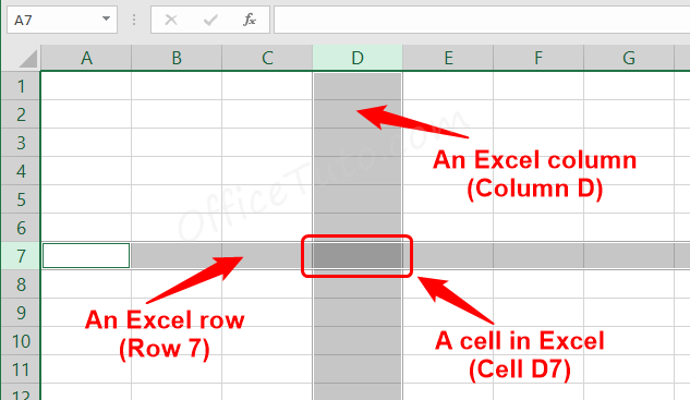
Excel worksheets have a tabular structure that is composed of columns, rows, and cells.

• Columns in Excel: A column refers to the vertical arrangement of cells. By default, it is labeled by a letter at the top of the column, such as A, B, C, etc.
• Rows in Excel: A row refers to the horizontal arrangement of cells. By default, it is labeled by a number on the left side of the row, such as 1, 2, 3, etc.
• Cells in Excel: A cell is the rectangular form created by the intersection of a row and a column. It is where you can enter, manipulate and store data.

By default, a cell in Excel is outlined in gray color. However, the outline won’t appear when the document is printed unless borders are applied to it (more on that later in the section “How to apply borders to Excel cells“).

2- How are rows and columns labeled in an Excel spreadsheet

There are two styles for labeling or referencing rows and columns in Excel: the default style (A1) and the R1C1 style.

• A1 style (the default style): In this style, rows are labeled with numbers and columns are labeled with letters. For example, the first column is labeled as “A,” the second column is labeled as “B,” and so on. The first row is labeled as “1,” the second row is labeled as “2,” and so on.
  So, as an example, the cell that belongs to column A and row 3 is referred to as “A3”.

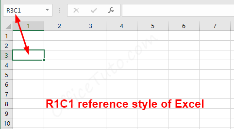
• R1C1 style: This style labels both rows and columns with numbers. The letters are replaced with numbers, where “R” represents rows and “C” represents columns.
  So, as an example, the cell that belongs to column 1 and row 3 is referred to as “R3C1”. See illustration below.

You can learn how to change the cell reference style in the “How to change the cell reference style of Excel” section below.

3- How many rows and columns are in an Excel spreadsheet

There are a total of 1,048,576 rows and 16,384 columns available in an Excel spreadsheet.

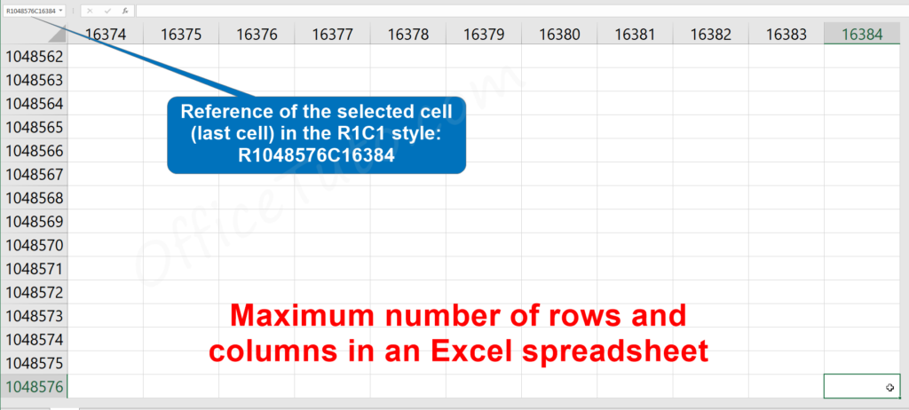
The rows are numbered from 1 to 1,048,576, while the columns are labeled from A to XFD (in the default reference style of Excel).

You can easily verify this by performing the following actions:

– To check the maximum number of rows: scroll down the vertical scroll bar to the bottom of the worksheet, and you’ll notice that the last row in the spreadsheet is labeled as 1048576.

You can also quickly check this in an empty spreadsheet by using the keyboard shortcut Ctrl + down arrow.

– To determine the maximum number of columns: a simple method is to enter the values “1” and “2” respectively in cells A1 and B1; then, select the cells and navigate to the “Editing” group within the “Home” tab of the ribbon. Click on the “Fill” drop-down, and select “Series”. Once the “Series” dialog box opens up, ensure that both “Rows” and “Linear” are checked, then click “OK”. Excel will automatically fill in the series from column A to XFD, and you can verify that the value of cell XFD1 is 16384.

Another way to find the total number of columns is to modify the reference style in Excel options from the default A1 to R1C1. This will change the labeling of the columns heading to numbers, and the heading of column XFD will appear as 16384.

You can also easily check this in an empty spreadsheet by using the keyboard shortcut Ctrl + right arrow.

4- Cell references in Excel

a- Reference of a single cell:

A cell reference is the address of a cell in an Excel spreadsheet, which is needed when using formulas or simply referring to a cell or a range of cells.

A cell’s reference is composed of its column letter and row number in the default referencing style. For instance, the first cell in a spreadsheet is called A1, representing the intersection of the first column A and the first row 1.

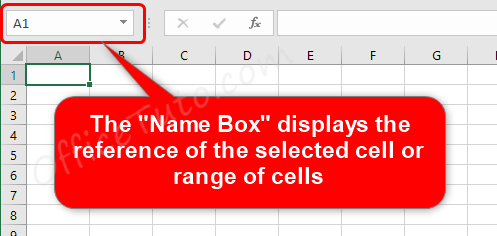
When you select a cell in Excel, its reference is displayed in the “Name Box,” which is located at the top-left corner under the ribbon.

b- Reference of a range of cells:

When you select a group of cells, known as a range of cells, its reference is created by the first cell, a colon, and the last cell. For instance, B1:D15 is the range of cells from B1 to D15.

c- How to change cell reference style of Excel

To change the cell reference style of Excel:

1. Click on “File” (or on the Office button in Excel 2007).
2. Click on “Options” (or “Excel Options” in Excel 2007.
3. “Excel Options” dialog box displays.
4. Click on “Formulas” from the left pane.
5. In the “Working with formulas” section, check or uncheck “R1C1 reference style”.
6. Click “OK“.

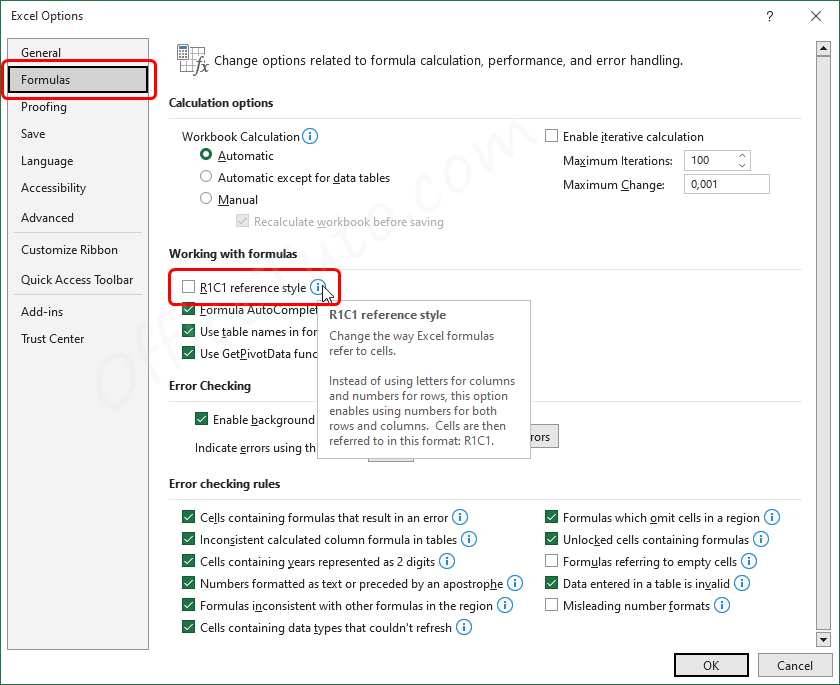
If you choose to check the “R1C1 reference style” option, both rows and columns will be labeled with numbers, and cells will be referenced with numbers only. For example, the cell from the third column and the fourth row will be referenced by R4C3.

If you prefer to use the default reference style, i.e., rows labeled with numbers and columns with letters, uncheck the “R1C1 reference style” option. For example, the cell from the third column and the fourth row will be referenced by C4.

5- Type of data and cell formats

Different types of data that can be entered in a cell include “text”, “numbers”, “dates”, and “formulas”.

Excel automatically selects the appropriate format for the data entered in a cell, whether it’s text format, number format, date format, currency format, percentage format, or others.

By default, it aligns text to the left and numbers and dates to the right in a cell.

Excel applies the following general formats when data is entered in a cell:

• The “Date” format when a date is entered in any of these formats: 01/02/2023, 01/02/23, 01-02-2023, or 01-02-23.
• The “Currency” format when a number is entered in the format $78.92 or $ 78.92.
• The “Percentage” format when a number is entered in the format 53.64% or 53.64%.
• The default “General” format for any other numeric and text data.

Excel automatically assigns the format to the data entered in a cell. However, if the format does not meet your requirements, you can manually assign a different format using the “Number Format” drop-down in the “Home” tab of the ribbon.

So, to assign or change a format of a cell in Excel:

1. Go to the “Home” tab of the ribbon.
2. Go to the “Number” group of commands,
3. Click on the “Number Format” drop-down list.
4. And select the format you need.

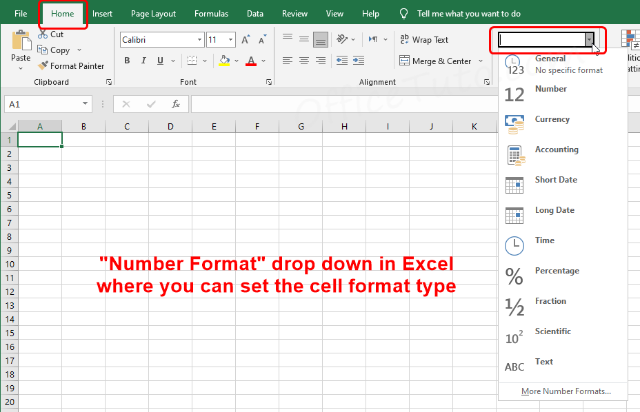
The “Number Format” drop-down list provides the following formats:

• General
• Number
• Currency
• Accounting
• Short Date
• Long Date
• Time
• Percentage
• Fraction
• Scientific
• Text
• And the “More Number Formats” option.

The last option, “More Number Formats”, provides you with additional options for special and custom formatting of the cells.

It’s worth noting that you can apply formatting to a cell either before or after you enter data into it.

If you’d like to learn more about Excel’s cell format types and how to utilize them effectively, I recommend checking out the tutorial on Cell Format Types in Excel.

6- How to enter data in Excel

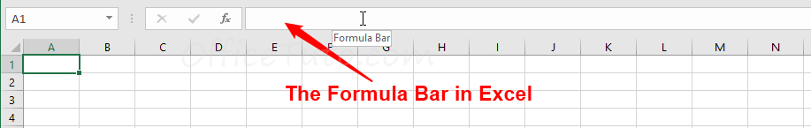
When adding data to Excel, you have two options: you can enter it directly into the cell or use the formula bar. Regardless of which method you choose, the data will be visible both in the cell and in the formula bar.

– To enter data directly in the cell: Click on the cell and start typing your content. When finished, simply hit Enter to complete the input.

– To enter data using the formula bar: First select the desired cell and then navigate to the formula bar. Enter your data there and press Enter to complete the process.

In my opinion, the formula bar is not necessary for small amounts of data input. However, if you need to enter a large amount of data into a cell with limited space, the formula bar may be useful.

7- How to edit data in Excel

To edit data that’s already entered in an Excel cell, there are two methods you can follow:

• Edit data in the cell itself:

Double-click on the cell containing the content you want to edit, then place your mouse cursor where you want to make the changes. Now, edit the content as desired and press Enter.

Note that there is a difference between editing the content in a cell and completely replacing it. If you just want to edit it, double-click on the cell and make the changes; but if you want to replace the entire content of the cell with new information, simply click on the cell (don’t double-click!) and type the new content.

• Edit data using the Formula Bar

Another way to edit the content of a cell is to use the formula bar. Simply select the cell you want to edit by clicking on it, then go to the “Formula Bar” and edit the content as desired (partially or completely). Finally, press Enter.

8- How to move between cells

To move between cells, you can either use the mouse by going to the desired cell and clicking on it, or by using the arrow keys of the keyboard (up, down, left, and right).

9- How to select entire rows or columns in Excel

a- How to select an entire row or column

There are 2 ways to select a whole row or column in Excel: using the mouse or using a keyboard shortcut.

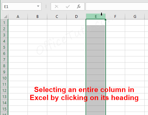
• Using the mouse:

To select an entire row or column in Excel using the mouse, click on its heading.

For instance, if you want to select column E, click on the letter “E” at the top of the column.

• Keyboard shortcut:

To select a whole row in Excel using the keyboard, click on a cell of this row, then press “Shift + Space“.

To select a whole column using the keyboard, click on a cell of this column, then press “Ctrl + Space“.

b- How to select multiple adjacent rows or columns

To select many rows or columns that are contiguous, you can click on the heading of the first row or column and, while holding down the left button of the mouse, select the others by going through their headings.

Alternatively, you can click on the heading of the first row or column, hold down the “Shift” key of the keyboard and click on the heading of the last row or column.

c- How to select multiple non-adjacent rows or columns

To select non-contiguous rows or columns in Excel, you need to select one row or column by clicking on its heading, then hold down the “Ctrl” key of the keyboard and select the other row or column, and so on.

10- How to change the formatting of the content of the cells

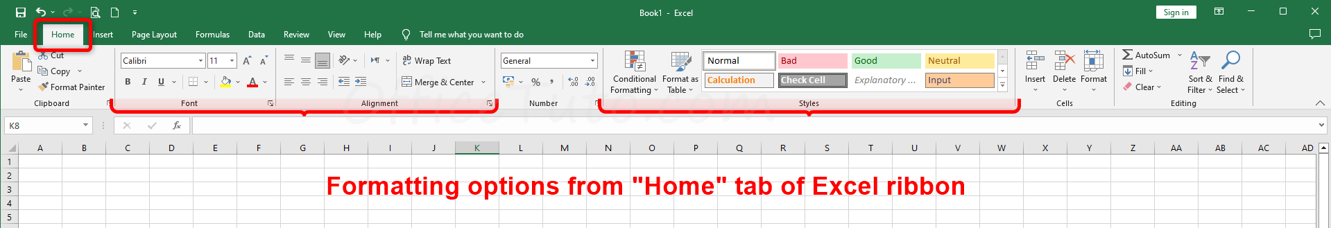
All data in Excel cells can be formatted using the formatting features in the “Home” tab of the ribbon, for the content of the selected cell, or for the cell itself.

This includes the font, the style of the font (Regular, Bold, Italic, Underlined…), the size of the content, the font color, the alignment of the content (Horizontal alignment and Vertical alignment), the indentation, the orientation of the content (rotation), and the fill color of the cell (color of the cell’s background); as well as some predefined styles for the cells.

You can access these options from the “Font“, “Alignment“, and “Styles” groups of commands in the “Home” tab of the ribbon.

To change the formatting of a cell or range of cells, simply select the cell or range of cells (or even a whole row, column, or many rows or columns, from their headings), and apply the desired formatting features.

Note: Keep in mind that you can always undo the changes if anything goes wrong, as well as redo them, using the respective commands “Undo” and “Redo” of the Quick Access Toolbar.

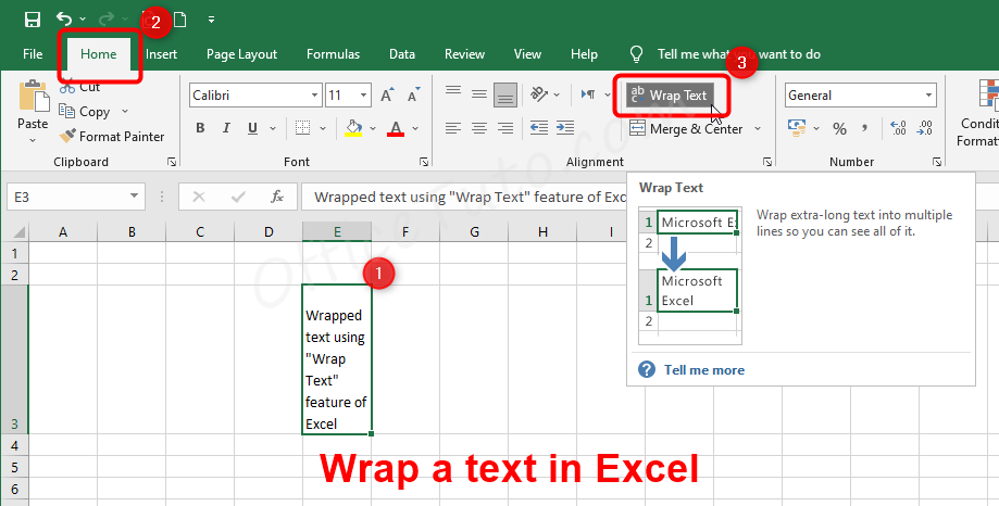
– How to wrap text in a cell

Wrapping text in a cell is making it in multiple lines in the same cell, without inserting a line break; the number of lines the text will display on will depend on the width of the column and the height of the row.

Now, to wrap a text in a cell, just select the cell and go to the “Alignment” group of commands in the “Home” tab of the ribbon. Then click on the “Wrap Text” command, and Excel will display the text according to the dimensions of the cell: its width and height.

11- How to change borders and background colors of cells

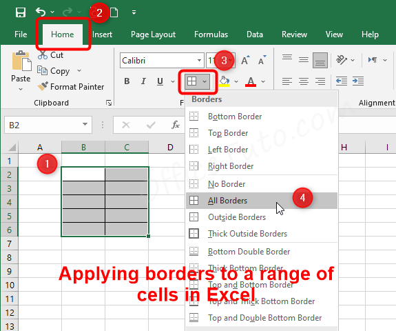
a- How to set or change cell borders

If you’re a beginner and work with an Excel sheet, you may think that the grid that constitues the cells is a real one and can be printed; well, this isn’t the case, and if you need a real table with printable borders, you need to apply these ones to your cells.

Fortunately, this is very easy:

So, to add borders to a range of cells, select the range and go to the “Borders” drop-down list in the “Font” group of commands of the “Home” tab of the ribbon. Choose the type of border you want to apply: “All Borders” would be a good start for you.

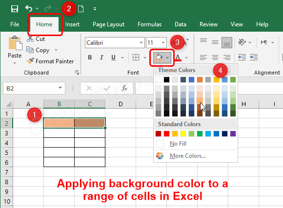
b- How to color cells background

To add a background color to cells, select them and go to the “Fill Color” drop-down list in the “Font” group of commands of the “Home” tab of the ribbon. Choose the desired color from the options available.

12- How to delete cell content

Deleting the content of an Excel cell is a quick and simple task. To do so, just click on the cell you want to clear, and press the “Delete” key on your keyboard.

The cell will be emptied, but it will remain in its place, ready to receive new data.

13- How to insert rows and columns

If you have a filled table and need to add new rows or columns, you can easily do so using one of the 3 methods available in Excel.

• Method 1: Right-click on the heading

To insert a row or column in Excel, simply right-click on the heading of the row or column where you want to insert a new one and choose “Insert” from the drop-down menu.

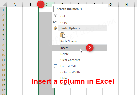
Excel will insert a new row above the selected row or a new column before the selected column, depending on your choice.

For example, if you want to insert a new column before Column C, right-click on the heading of Column C and select “Insert” from the menu. Excel will insert a new column before Column C.

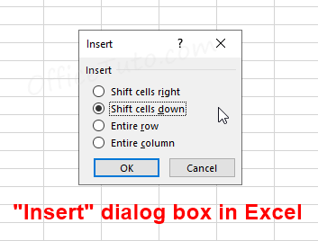
• Method 2: “Insert” dialog box

Apart from the first method, you can also insert a row or column by right-clicking on a cell in the row or column where you want to insert a new one, and use the options provided by the “Insert” dialog box.

• Method 3: “Insert” drop-down from the ribbon

Alternatively, you can use the “Insert” drop-down list from the “Home” tab of the ribbon.

14- How to insert cells

In order to insert cells in an already populated Excel table, you may need to add new items that were not originally planned, but inserting an entire row or column will disrupt the organized data in other tables. To avoid this, you can insert cells instead. Here’s how:

• To insert a single cell:

Right-click on the cell above the position where you want to insert the new one, then click on “Insert“. In the “Insert” dialog box that displays, choose one of these 4 options, depending on your needs: Shift cells right, Shift cells down, Entire row, or Entire column.

• To insert multiple cells:

Go to the position where you want to insert the cells, then select above it the same number of cells you want to insert. Right-click on the selection, and then click on “Insert“. In the “Insert” dialog box that displays, choose one of these 4 options, depending on your needs: Shift cells right, Shift cells down, Entire row, or Entire column.

Keep in mind that inserting new cells in an Excel table may result in changes to the existing tables on the same sheet, so you may need to perform additional tasks like merging cells or moving them.

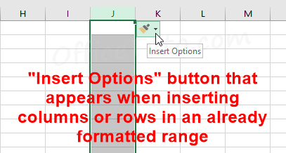
Formatting options when inserting

When you insert a new row or column in Excel and have a specific formatting applied in any of the adjacent cells, the formatting of the adjacent rows, columns, or cells may be automatically applied to the newly inserted one. If you do not want this to happen, you can select the “Insert Options” button that appears after insertion, and then choose one of the provided options to keep same formatting or clear it.

15- How to delete rows, columns, or cells

a- How to delete rows and columns in Excel

To delete a row or column in Excel, you can use one of three methods: right-clicking on the heading, right-clicking on a cell, or using the ribbon.

• Method 1: Delete a row or column by right-clicking on its heading

To delete a row or column, simply right-click on the heading of the row or column you want to delete and select “Delete”. Excel will then remove the selected row or column.

• Method 2: Delete a row or column by right-clicking on a cell

Another way to delete a row or column is by right-clicking on any cell within the row or column you want to remove, selecting “Delete”, and then choosing “Entire Row” or “Entire Column” in the dialog box that appears. Click “OK” to confirm.

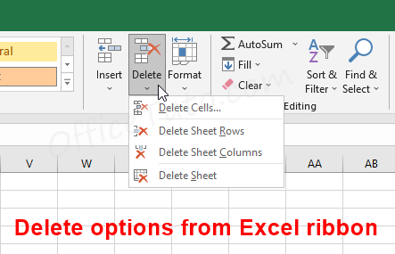
• Method 3: Delete a row or column using the ribbon

Finally, you can delete a row or column using the “Delete” command in the “Cells” group on the “Home” tab of the ribbon. Select the cell in the row or column you want to delete, click on “Delete”, and then choose “Delete Sheet Rows” or “Delete Sheet Columns” as appropriate.

b- How to delete cells in Excel

Deleting the cell itself is different from deleting just its content, as the latter will leave empty cells in the table. Unlike clearing the contents of a cell, deleting a cell means that it will no longer exist, along of course with its content; but there will be no empty space in the grid as Excel will fill this space with another cell by shifting the other cells in the way the user wants.

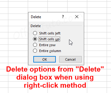
My prefered way to delete cells in Excel is by using the right-click.

So, to do that, just select the cell or range of cells you want to delete. Right-click on the selection and click on “Delete“. In the “Delete” dialog box that displays, choose one of these 4 options, depending on your needs: Shift cells left, Shift cells up, Entire row, or Entire column.

Excel will delete the selected cells. However, be cautious when deleting cells as it can cause disorder in your table. If this happens, you may need to merge some cells or undo the deletion of the cells and delete only their content. In any case, you’ll know what to do!

16- Units of row height and column width

a- Row height unit

In Excel, row height is measured using different units depending on the view.

The Normal view uses Points, while the Page Layout view uses Inches:

• In the Normal view: Excel row height is calculated in points. One point is equivalent to 1/72 inches or about 1.33 pixels in a 96 DPI configuration.
• In the Page Layout view: Excel row height is measured in inches by default, although it can be changed to centimeters or millimeters in Excel options.

b- Column width unit

Similar to the row height, Excel uses different units for the column width in the Normal and Page Layout views.

Excel column width unit is Characters in the Normal view and Inches in the Page Layout view:

• In the Normal view: The unit for the column width is Characters, specifically zero characters, which represents how many of them can fit in a single line.
• In the Page Layout view: Excel column width is measured in inches by default. Just like with row height, the unit can be changed to centimeters or millimeters in Excel options.

For detailed information on units of row height and column width in Excel, see the dedicated tutorial What Are Units of Column Width and Row Height in Excel.

17- The default row height and column width in Excel

In Excel, the width of a column and the height of a row determine their respective sizes.

The size of a cell is determined by the width of its column and the height of its row.

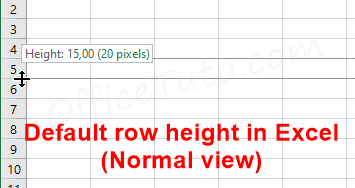
• In the “Normal” view, the default row height in Excel is 15 points, while in the “Page Layout” view with 100% scaling, it is 0.21 inches.

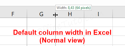
• The default column width in the “Normal” view is 8.43 characters, specifically 8.43 of zero characters, for the default font and size (Calibri – size 11).
  In the “Page Layout” view with 100% scaling, the default column width is 0.72 inches.

To understand more the different units used for row height and column width in Excel, see the dedicated tutorial What Are Units of Column Width and Row Height in Excel.

If these default measures don’t suit your needs and you want to change them, you can check the advanced tutorial How To Set a New Default Column Width and Row Height in Excel.

18- How to change the row height and column width in Excel

a- How to change column width in Excel

The simplest way to adjust the width of one or more columns in Excel is to use the drag and drop of the mouse.

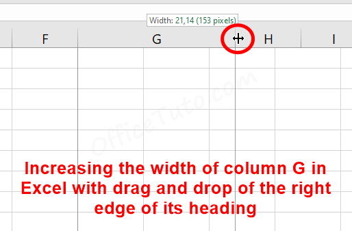
To adjust a column’s width in Excel using the drag and drop of the mouse:

• Position the cursor on the right edge of the column’s header.
• The cursor will change to a double-sided arrow.
• Click and hold the left mouse button while dragging the right edge to the right to increase the width, or to the left to decrease it.

In the example illustrated below, I’m increasing the width of column G using this method:

For more detailed information on how to change the width of a column in Excel, refer to the section How To Change Columns Width in Excel from the tutorial How To Change the Columns Width and Rows Height in Excel.

b- How to change row height in Excel

Changing the height of a row in Excel is very similar to changing the width of a column.

I will show you here the easiest technique for dynamically adjusting row height in Excel, which is to use the drag and drop of the mouse.

To adjust a row’s height in Excel using the drag and drop of the mouse:

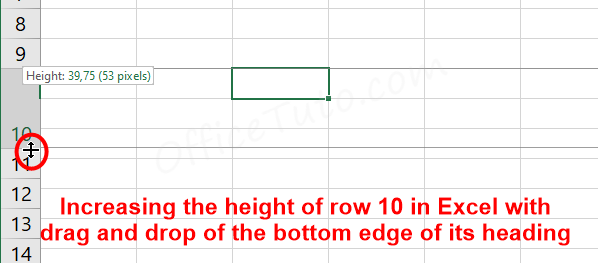
• Place the cursor on the bottom edge of the row’s header.
• The cursor will change to a double-sided arrow.
• Click and hold the left mouse button while dragging the bottom edge to the bottom to increase the height, or to the top to decrease it.

In the example illustrated below, I’m increasing the height of row 10 using this method:

For more detailed information on how to change the height of a row in Excel, refer to the section How To Change Rows Height in Excel from the tutorial How To Change the Columns Width and Rows Height in Excel.

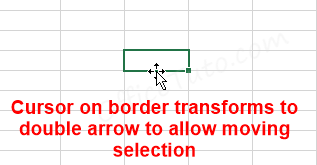
19- How to move cells, rows and columns

To move cells, rows, or columns in Excel, first select them (for rows or columns, select them by their headings), then place the mouse cursor on the border of the selection. The cursor will change into a double-arrow shape. You can then drag the selection to the desired location.

20- How to merge cells in Excel

a- How to merge cells

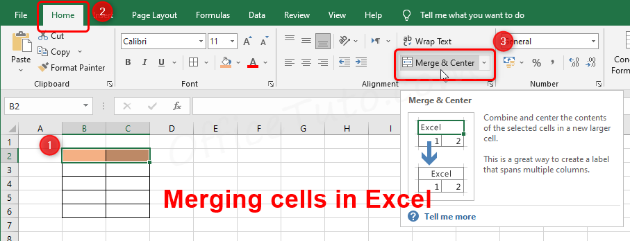
Merging cells in Excel is useful when you want to combine the contents of two or more cells into one.

To merge cells, select the cells you want to merge, then go to the “Home” tab of the ribbon. In the “Alignment” group of commands, click on “Merge & Center“.

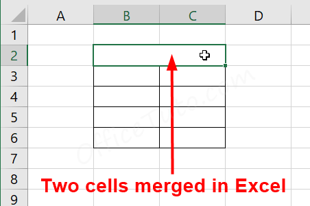
If the upper-left cell and another one(s) contain data, Excel will first warn you by a message that all content will be removed except for the content of the upper-left cell.

In the following illustration, you can see an example of two merged cells in Excel:

b- How to unmerge cells

If you have already merged cells and need to unmerge them, the process is also straightforward.

So, to unmerge cells, select the merged cells you want to unmerge, and click on the “Merge & Center” command again from the “Alignment” group of commands in the “Home” tab of the ribbon.

As you notice, this tool has a double effect: it can both merge and unmerge cells.

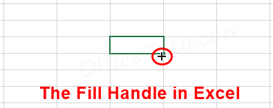
21- Use the Fill Handle to copy content to adjacent cells or fill a series

The fill handle in Excel is the black plus sign form that the mouse cursor takes when hovering over the lower-right corner of a selected cell or selection of cells.

a- Copy content to adjacent cells using the fill handle

When you want to quickly copy cell content to adjacent cells, you can use Excel’s fill handle instead of copy and paste commands.

To copy content to adjacent cells using the fill handle, select the cell or range of cells you want to extend the content, then put the mouse over the lower-right corner of the cell or selection of cells, and click and drag the fill handle to extend the content to the desired range of cells.

b- Extend a series using the fill handle

You can also use the fill handle to continue a series in Excel. If you have a sequence of numbers, days of the week, months, dates, or alphanumeric text, Excel can predict what comes next in the series.

• To continue a series of numbers: you’ll need to fill the first and second cell, select them both, then click and drag the fill handle of the selection to extend the series.
  
• To continue a series of days of the week, months, dates, or alphanumeric text: you don’t have to fill a second cell; Excel will understand itself that this will be a series.
  So, select this first cell, then click and drag the fill handle of the cell to extend the series.

With large spreadsheets, it would be better to automatically fill the series by double-clicking the fill handle, instead of dragging the mouse across a huge number of rows or columns.

22- How to copy the size of the columns or rows in Excel

a- How to copy columns width in Excel

Copying the size of columns or rows in Excel can be done in three ways: copy-pasting, using the Format Painter tool, or utilizing the Paste Special feature.

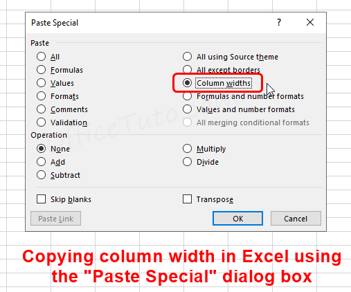
I will show you here how to copy the width of columns in Excel using the Paste Special feature. Here are the steps:

1. Select the heading(s) of the column(s) that you want to copy the width of.
2. Press Ctrl + C or click the “Copy” command in the “Home” tab.
3. Navigate to the target column(s) where you want to apply the copied column width.
4. Right-click on the column heading and select “Paste Special“.
5. The Paste Special dialog box will appear.
6. Check the “Column widths” option and click OK.
7. Excel will apply the width of the source column(s) to the destination column(s).

To check the other two methods and get more information about this topic, go to the other tutorial: How to copy columns width in Excel.

b- How to copy rows height in Excel

There are 2 methods of copying rows height in Excel: by either using the copy paste, or through the Format Painter tool.

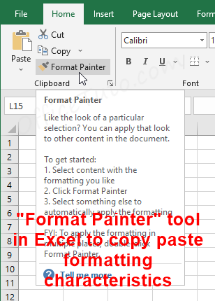
I will show you here how to use the Format Painter tool to copy rows height. Here is how to do it:

1. Select the heading(s) of the row(s) you want to copy the height.
2. Go to the “Clipboard” group of commands in the “Home” tab.
3. Click on the “Format Painter” tool.
4. Go to the target rows where you want to apply the same row height.
5. Select the entire row(s) by the heading(s).
6. Excel will apply the same height and formatting of the source row(s) to the destination one(s).

To check the other methods and get more information about this topic, go to the other tutorial: How to copy rows height in Excel.

23- How to sort columns and rows in Excel

Sorting data in Excel can be incredibly useful when working with numbers, dates, or text. To sort your data in Excel, follow these simple steps:

1. Click on a cell from the range of cells you want to sort.
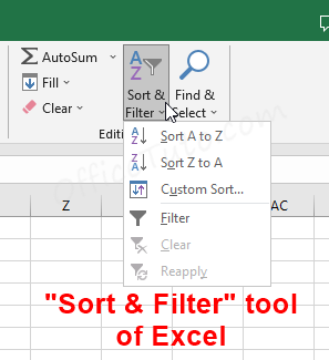
2. Go to the “Home” tab of the ribbon and click on the “Sort & Filter” drop-down list in the “Editing” group of commands. Then, choose the option you need.
   Alternatively, you can go to the “Data” tab of the ribbon, and choose the option you want in the “Sort & Filter” group of commands.
3. You’ll notice that Excel automatically detects the format of data to sort and provides the right sorting commands accordingly:
   – If you have text data (or text mixed with numbers), the commands will show “Sort A to Z” and “Sort Z to A”.
   – For numbers, the commands will show “Sort Smallest to Largest” and “Sort Largest to Smallest”.
   – For dates, the commands will show “Sort Oldest to Newest” and “Sort Newest to Oldest”.

This was the basic use of the sorting feature in Excel. For more detailed information, you can check out the dedicated tutorial “How to sort data in Excel“.

24- How to freeze columns and rows in Excel

When working with Excel spreadsheets that have extensive information, it’s common to encounter situations where the data extends beyond the visible screen area. Scrolling through the sheet using the arrow keys or scroll bars is a typical solution, but it can lead to losing sight of important column and row headers that provide context.

To address this concern, Excel offers a feature called “Freeze Panes” that allows you to keep specific rows and columns visible on the screen at all times, even when scrolling through the remaining data.

To freeze columns and rows in Excel, follow these steps:

1. Position the cursor in the cell located below the row(s) and to the right of the column(s) you want to freeze. This cell acts as a reference point for the freezing process.
2. From the Excel ribbon, navigate to the “View” tab.
3. In the “Window” group of commands, click on the “Freeze Panes” drop-down list.

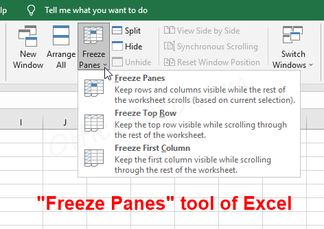
4. From the options presented, choose either “Freeze Panes” to freeze both columns and rows up to the selected cell, or select “Freeze Top Row” or “Freeze First Column” to freeze only the top row or the leftmost column, respectively.

Excel will now freeze the designated columns and rows, ensuring they remain visible regardless of any scrolling performed within the sheet. This helps maintain important headers in view, enabling better comprehension of the presented information.

Remember, if you wish to remove the frozen panes and revert to the normal scrolling behavior, access the “Freeze Panes” drop-down list from the “View” tab and select the “Unfreeze Panes” option.

I have detailed this in more detailed aspect, with illustrated examples, in the advanced tutorial “How to freeze rows and columns in Excel“.

25- How to filter data in Excel

Filtering data in Excel is an incredible feature that allows you to display a specific part of your data based on chosen criteria. Let me guide you through the process:

1. Start by selecting any cell within your data list.
2. To access the filtering options, you have two methods:
   • Go to the “Home” tab of the ribbon and click on the “Sort & Filter” drop-down list in the “Editing” group of commands. Choose “Filter“.
   • Alternatively, go to the “Data” tab and click on the “Filter” command in the “Sort & Filter” group of commands.
3. Excel will immediately add vertical arrows as filters on each column header of your data.
4. To apply a specific criterion and filter your data, click on the arrow next to the column containing the criterion you want to use. Excel will display a drop-down list as illustrated below:

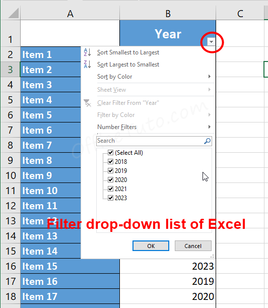
5. In the drop-down list, uncheck all options except for the desired criterion, such as “my criterion”. Click OK.
6. Excel will instantly filter your data based on the chosen criterion and display a “Filter icon” on the filtered column’s arrow.
7. You can easily identify if a filter is applied and on which column by observing the highlighted “Filter” command, arrows on column labels, and any numbering gaps in the row headings.
8. To remove the filter and display the entire data again, simply click on the same “Filter” command in the “Home” or “Data” tabs.

This was a quick overview of the filter feature in Excel. I explained all of this, in more detailed and advanced aspect, in the dedicated tutorial “How to filter data in Excel“.

26- How to hide columns and rows in Excel

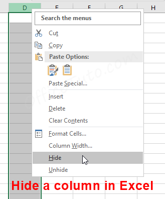
• To hide a column in Excel:

To hide a column using the right-click option, select the entire column, by clicking on its heading, then right-click on the selection, and choose “Hide” from the context menu.

• To hide a row in Excel:

Select the entire row you want to hide, by clicking on its heading, then right-click on the selection and choose the “Hide” option.

• To unhide a hidden column in Excel:

To unhide a hidden column using the right-click option, select the two columns surrounding the hidden column, right-click on the selection, and select “Unhide.”

• To unhide a hidden row in Excel:

Select the two rows surrounding the hidden row, then right-click on the selection and select “Unhide” from the menu.

27- How to convert rows to columns or columns to rows in Excel

If you have values arranged in rows in your Excel workbook and want to convert them to columns, there are a few methods you can use.

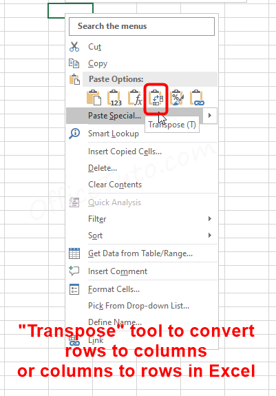
The easiest way is to utilize the Paste Transpose option.

Let’s take the example of converting rows to columns:

1. Select and copy the range of cells belonging to the rows you want to convert.
2. Right-click on the cell where you want the transposed columns to begin.
3. Choose the Paste Transpose option, which rotates the rows into columns.

Alternatively, you can use the Paste Special option and select the Transpose option.

The same process applies when converting columns to rows in Excel.

– Wrap up

That was my beginner tutorial on rows, columns, and cells in Excel.

By reading this tutorial and applying all its steps, I think you’ll have a thorough comprehension of these fundamental elements and be fully equipped to effectively handle more advanced Excel techniques with confidence.