How To Change the Columns Width and Rows Height in Excel

Whenever you work on an Excel spreadsheet, in most cases you will need to change the size of the cells to be able to view all the content they contain. But, to do this, and due to the tabular structure of the spreadsheet, you will of course have to resize the entire column or row to which the cell belongs.

In the following, I will show you how to know the current size of a column or row, what are the minimum and maximum sizes of a cell, how to resize a column or a row (with examples), and how to make multiple columns or rows the same size (with examples). I will also discuss the issue that is sometimes caused by the autofit feature of Excel compared to the manual resizing of columns width and rows height, and how to solve it.

So, let’s now start with how to actually know the current width of a column or height of a row.

A/ How to know the column width or row height in Excel

1- How to know the current width of a column in Excel

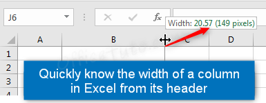
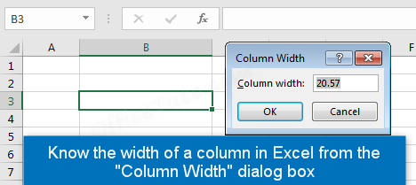
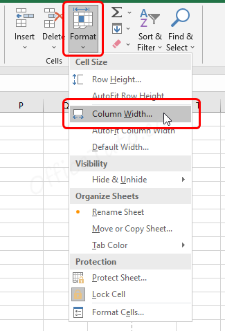
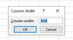
To know the width of a column in Excel, hold down the click on the right boundary of its header, and Excel displays its width in a tooltip. Or, click a cell of the column; go to “Home” tab and click “Format” drop-down of the “Cells” group, then click “Column Width”. Excel displays the width of the column in the “Column Width” dialog.

Or

The unit of the column width is in characters; i.e., how many zero characters fit in this width in one line, in the “Normal” view, for the default font and size (Calibri – size 11). For more insight on how the columns width is calculated and on its unit, check What Are Units of Column Width and Row Height in Excel.

In my opinion, even though the first method of clicking the right boundary of a column header to display the tooltip is faster to find the current column width, but it may lead to unintentionally drag the mouse to the right or left side, which will change the width of the column. I prefer to use the “Format” dropdown method when I don’t want the current structure of my columns to be affected.

2- How to know the current height of a row in Excel

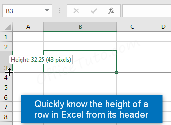
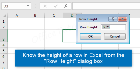
To know the height of a row in Excel, hold down the click on the bottom boundary of its header, and Excel displays its height in a tooltip. Or, click a cell of the row; go to “Home” tab and click “Format” drop-down of the “Cells” group, then click “Row Height”. Excel displays the height of the row in the “Row Height” dialog.

Or

The unit of the row height is in points. For more in-depth information on how the rows height is calculated and on its unit, check What Are Units of Column Width and Row Height in Excel.

As you may notice, the first method of clicking the right boundary of a row header to display the tooltip is faster to find the current row height, but it may lead to unintentionally drag the mouse to the top or bottom side, which will change the height of the row. I think that using the “Format” dropdown method is better when you don’t want the current structure of your rows to be affected.

B/ Minimum and maximum sizes of cells in Excel

1- Minimum and maximum column width in Excel

The column width in the normal view of Excel is calculated in characters (how many zero characters fit in).

The minimum size of a column width in Excel is 0, which is the equivalent of hiding the column.

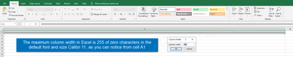
The maximum size of a column width in Excel is 255 characters (255 of zero characters) in the “Normal” view, for the default font and size (Calibri – size 11); or 20.03 inches in the “Page Layout” view (for a 100% scaling).

In the Normal view, the 255 characters is not the number of characters a cell can contain (a cell can contain up to 32,767 characters); it’s the maximum number of characters (zero characters) a column can show in its width in one line. If there are more characters, they will just overflow to the right of the cell in the same line, or to more lines if the wrap text feature is applied.

In the example illustrated below, I show you how the maximum column width in Excel fits with 255 of zero characters, in the default font and size Calibri 11.

Of course, when you change the font, the size, or the style (Bold, Italic), the maximum number of characters a column can show in its width in one line will change.

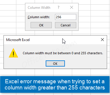
If you try to set a column width greater than 255 characters, Excel will refuse and display an error message; see the screenshot below.

2- Minimum and maximum row height in Excel

The row height in the normal view of Excel is calculated in points.

The minimum size of a row height in Excel is 0, which is the equivalent of hiding the row.

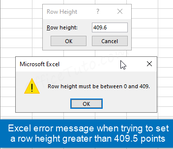
The maximum size of a row height in Excel is 409.5 points in the “Normal” view, or 5.69 inches in the “Page layout” view (for a 100% scaling).

Now, after learning how to know the current width of a column and height of a row, as well as learning the minimum and maximum sizes allowed in Excel, let’s see how to change this column width or row height in Excel.

C/ How to resize a column in Excel

The default column width in Excel is 8.43 characters (8.43 of zero characters) in the “Normal” view, for the default font and size (Calibri – size 11); or 0.72 inches in the “Page Layout” view (for a 100% scaling).

So, when you create a new spreadsheet, columns will have the default width; but you can of course change this width to the size you want.

Note also that you can set a new default width for columns in Excel; I detailed this in How To Set a New Default Column Width and Row Height in Excel.

Let’s see now how to change the column width in Excel.

There are 3 ways to resize columns in Excel:

1. Dynamically, through the mouse drag and drop.
2. Precisely, via the right click or the ribbon.
3. Automatically fit the content of the cells (Autofit).

I will detail each method in the following sections:

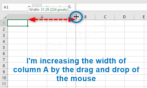
1- How to resize columns in Excel with drag and drop

In this first method of resizing a column or multiple columns in Excel, I will use the drag and drop of the mouse.

To resize a column in Excel using the drag and drop of the mouse:

1. Place the cursor on the right boundary of the column’s heading.
2. The cursor is transformed to a double-sided arrow.
3. Click and drag this right boundary to the right to widen the column, or to the left to narrow it.

To resize multiple columns in Excel using the drag and drop of the mouse:

1. Select first the columns by their headings.
2. Place the cursor on a boundary of any of these headings.
3. The cursor is transformed to a double-sided arrow.
4. Click and drag this boundary to the right to widen the columns, or to the left to narrow them.
5. Excel changes the width of all selected columns.

2- How to precisely resize columns in Excel via the dialog box

You can resize a column or multiple columns in Excel with a precise size, using the right click or the ribbon.

a- How to precisely resize columns in Excel using the ribbon

I will use here the “Column Width” dialog box displayed from the ribbon, to enter a precise value of the width I want.

To resize with a precision a column or multiple columns in Excel using the ribbon:

1. Select the column or columns by the heading(s).
2. Go to the “Cells” group of the “Home” tab.
3. Click “Column Width” in the “Format” drop-down.
4. Excel displays the “Column Width” dialog box.
5. Set precisely the column width you want.
6. Click OK to apply the new width.

b- How to precisely resize columns in Excel using the right click

I will use here the “Column Width” dialog box displayed with the right click, to enter a precise value of the width I want.

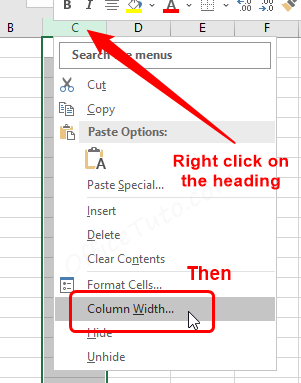
To resize with a precision a column or multiple columns in Excel using the right click:

1. Select the column or columns by the heading(s).
2. Right-click the selection.
3. Choose “Column Width” from the menu.
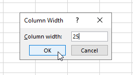
4. Excel displays the “Column Width” dialog box.
5. Set precisely the column width you want.
6. Click OK to apply the new width.

Note: The actual number of characters displayed within the width of the columns (in one line) depends of course on the font, size and style used.

3- Automatically adjust columns width in Excel to fit the content

The above methods of adjusting cell width work well for manual adjustments; however often times when adjusting the cell width, the goal is to be able to see all the content within that cell. When that is the desired goal, there is a quicker and automatic solution, and the end result is more consistent.

There are two ways to automatically adjust columns width in Excel:

• With the double click of the mouse.
• Through the autofit command from the ribbon.

a- Auto-adjust columns width in Excel with the double click

I will use here the first method of automatically adjusting columns width in Excel, which is using the double click of the mouse. I will apply it on a single column, as well as on multiple columns.

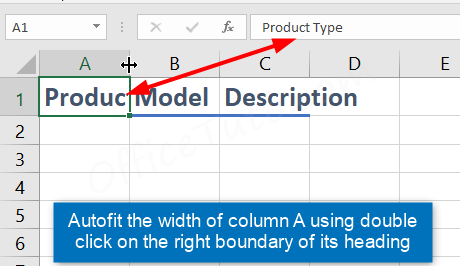
So, to automatically adjust one column width in Excel to fit the content of its cells:

1. Place the cursor on the right boundary of the column heading.
2. The cursor changes to a double-sided arrow.
3. Double-click the mouse.
4. Excel will automatically size the column to fit the largest content of its cells.

In the example of the screenshot below, the content of cell A1 is not entirely visible, so I use the double click on the heading of column A to autofit its width.

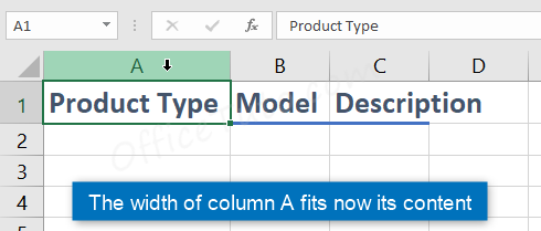
Here is the result after applying the autofit with double click on column A:

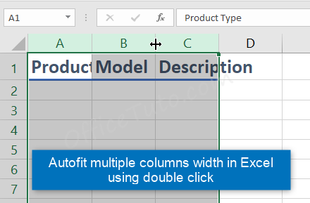
On the other hand, to automatically adjust the width of multiple columns in Excel to fit the content of their cells:

1. Select the columns through their headings.
2. Place the cursor on a boundary of any of these headings
3. The cursor changes to a double-sided arrow.
4. Double-click the mouse.
5. Excel will automatically size each column to fit the largest content of its cells.

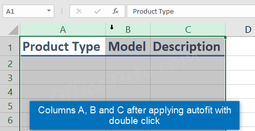
Here is the result after applying the autofit with double click on columns A, B and C:

b- Automatically adjust cells or columns width in Excel via the ribbon

This is the second method of automatically adjusting cells or columns width in Excel, which is via the ribbon commands. I will show you how to autofit one cell or multiple cells width, as well as one or multiple columns width.

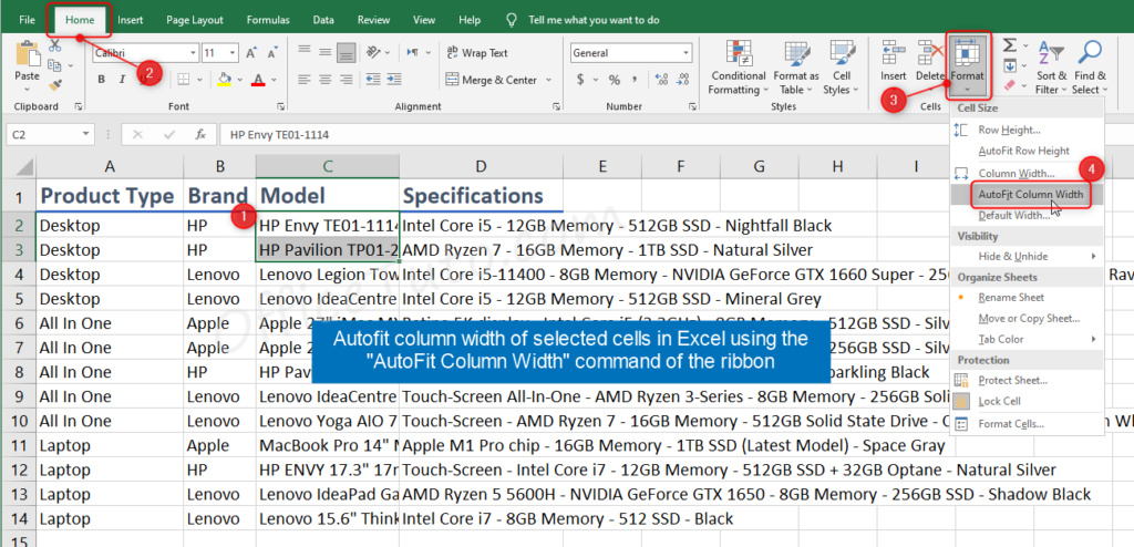
b1- Autofit one or multiple cells width in Excel using the ribbon

The ribbon command I will use here to autofit my cells is the “AutoFit Column Width” format command.

To automatically adjust one or multiple cells width in Excel to fit its content, using the ribbon:

1. Select the cell or cells you want to autofit the width.
2. Go to the “Cells” group of the “Home” tab.
3. Click in the “Format” drop-down on “AutoFit Column Width”.
4. Excel automatically adjusts the width of the column to fit the content of the selected cell or cells.

Note: If the content of any other cells is larger than the new size of the column, it will overflow to their right cell.

In the following example, I want to autofit the width of cells C2 and C3, because their width suits my needs, but not the other cells of column C that contain too long content, because of limited workspace; so, I preferred to apply the wrap text feature to these other cells, and autofit the first two cells of the column.

The result of applying the “AutoFit Column Width” format command on the selection of cells C2:C3 is illustrated below:

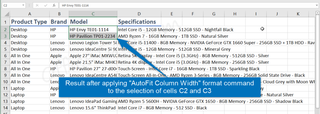
As you can see, the width of column C is adjusted to fit the content of the largest cell in the selection, which is cell C3 in my example. If there are any cells with a content longer than the width of C3, it will overflow to the next cell on the right if this cell is empty, or its extra will be hidden as you see in the screenshot above for the range C4:C14.

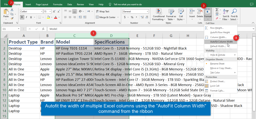
b2- Autofit one or multiple columns width in Excel using the ribbon

I will use here the “AutoFit Column Width” format command to autofit my columns.

To automatically adjust one or multiple columns width in Excel to fit the content, using the ribbon:

1. Select the columns you want to autofit. If it’s just one column, you can simply click on a cell from it.
2. Go to the “Cells” group of the “Home” tab.
3. Click in the “Format” drop-down on “AutoFit Column Width”.
4. Excel automatically adjusts the width of the selected column or columns, to fit the largest content of its or their cells.

The result of applying the “AutoFit Column Width” command on the selected columns C and D is illustrated below:

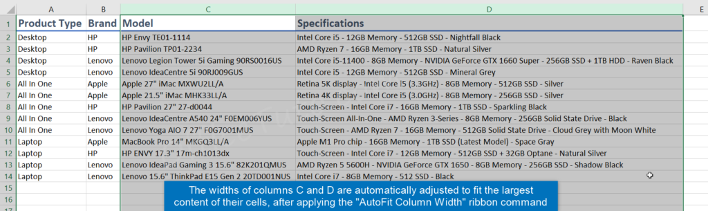
As you can see, the width of column C is adjusted to fit the content of cell C14 (cell with the largest content in column C), and the width of column D is adjusted to fit the content of cell D4 (cell with the largest content in column D).

D/ How to resize a row in Excel

Often times, you’ll need to resize a row (or rows) in Excel when the text contained in it is wrapped or when there are multiple lines in the same cell.

The default row height in Excel is 15 points in the “Normal” view, or 0.21 inches in the “Page Layout” view (for a 100% scaling).

So, when you create a new spreadsheet, rows will have the default height; but you can of course change this height to the size you want.

Note also that you can set a new default height for rows in Excel; I detailed this in How To Set a New Default Column Width and Row Height in Excel.

Let’s see now how to change the row height in Excel.

There are 3 ways to resize rows in Excel:

1. Dynamically, through the mouse drag and drop.
2. Precisely, via the right click or the ribbon.
3. Automatically fit the content of the cells (Autofit).

I will detail each method in the following sections:

1- How to resize a row in Excel dynamically via drag and drop

I will show you here the first method of dynamically adjusting rows height in Excel, which is using the drag and drop of the mouse.

To resize a row in Excel using the drag and drop of the mouse:

1. Place the cursor on the bottom boundary of the row’s heading.
2. The cursor is transformed to a double-sided arrow.
3. Click and drag this bottom boundary to the bottom to widen the row, or to the top to narrow it.

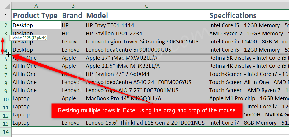
To resize multiple rows in Excel using the drag and drop of the mouse:

1. Select first the rows by their headings.
2. Place the cursor on a boundary of any of these headings.
3. The cursor is transformed to a double-sided arrow.
4. Click and drag this boundary to the bottom to widen the rows, or to the top to narrow them.
5. Excel changes the width of all selected rows.

In the example illustrated below, I’m increasing the height of rows 2 to 13 using the drag and drop of the mouse.

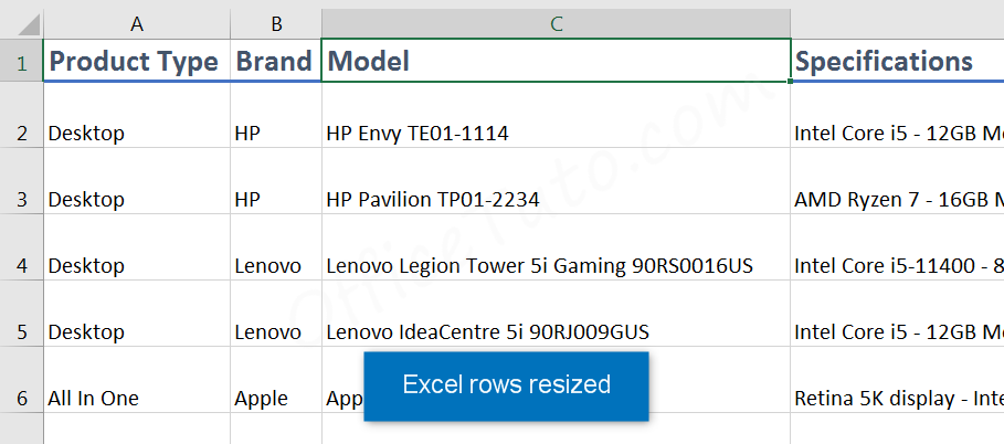
Here is the result:

2- How to precisely resize rows in Excel via the dialog box

You can resize a row in Excel with a precise size that you can enter manually, using the right click or the ribbon.

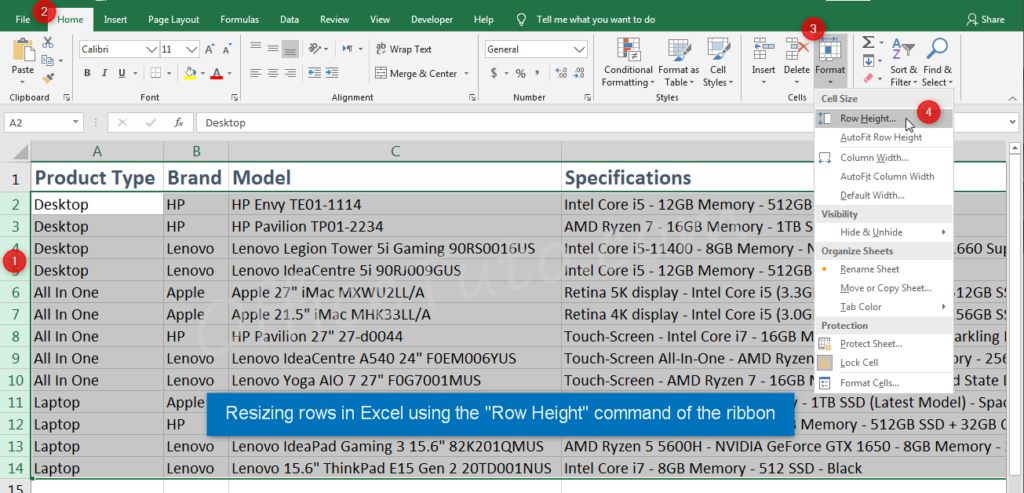
So, to resize with a precision a row or multiple rows in Excel using the ribbon:

1. Select the row or rows by the heading(s).
2. Go to the “Cells” group of the “Home” tab.
3. Click in the “Format” drop-down on “Row Height”.
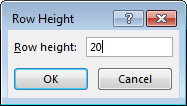
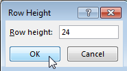
4. Excel displays the “Row Height” dialog box.
5. Set how many points you want as a row height.
6. Click OK to apply the new height.

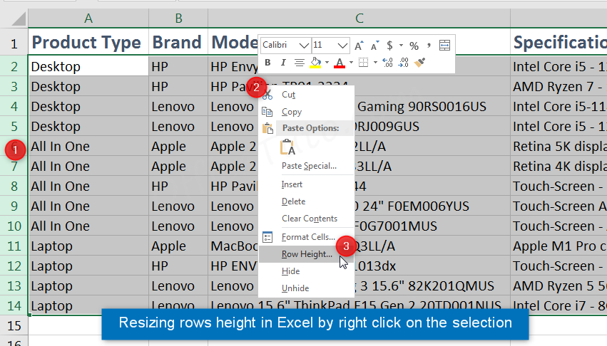
To resize with a precision a row or multiple rows in Excel using the right click:

1. Select the row or rows by the heading(s).
2. Right-click the selection.
3. Choose “Row Height” from the menu.
4. Excel displays the “Row Height” dialog box.
5. Set how many points you want as a row height.
6. Click OK to apply the new height.

3- Automatically adjust rows height in Excel to fit the content

The above methods of adjusting cell height work well for manual adjustments as you control yourself the row size; however, when you want to fit the row height to its content, there is a quicker and automatic solution, that will give you a more precise result.

However, there is one condition for the autofit to work on the row(s): a manual adjustment must have been applied beforehand on the row(s) for the autofit to be effective and be able to correct the manual adjustment.

There are two ways to automatically adjust rows height in Excel:

• With the double click of the mouse.
• Through the autofit command from the ribbon.

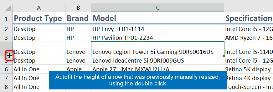
a/ Auto-adjust rows height in Excel with the double click

I will use here the first method of automatically adjust rows height in Excel, which is using the double click of the mouse.

So, to automatically adjust one row height in Excel to fit the content of its cells, provided of course that a manual adjustment was previously applied on:

1. Place the cursor on the bottom boundary of the row heading.
2. The cursor changes to a double-sided arrow.
3. Double-click the mouse.
4. Excel will automatically size the row to fit the longest wrapped or multi-line content of its cells.

On the other hand, to automatically adjust the width of multiple rows in Excel to fit the content of their cells, provided of course that a manual adjustment was previously applied on:

1. Select the rows through their headings.
2. Place the cursor on a boundary of any of these headings.
3. The cursor changes to a double-sided arrow.
4. Double-click the mouse.
5. Excel will automatically size each row to fit the longest content of its cells.

b/ Automatically adjust cells or rows height in Excel via the ribbon

This is the second method of automatically adjust cells or rows height in Excel, which is via the autofit command of the ribbon.

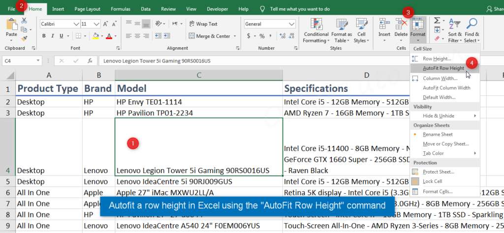
So, to automatically adjust one cell or row height in Excel to fit its content, using the ribbon:

1. Select a cell from the row.
2. Go to the “Cells” group of the “Home” tab.
3. Click in the “Format” drop-down on “AutoFit Row Height”.
4. Excel automatically adjusts the height of the row to fit the longest content of the row cells.

In the example below, I’m applying the “AutoFit Row Height” command on row 4 (a row that was manually adjusted previously):

The result is illustrated below:

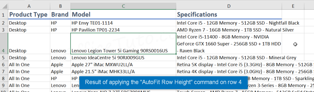
As you can see, the row height was automatically adjusted to fit the longest content of its cells, which is the content of cell D4.

To automatically adjust multiple rows height in Excel to fit the content, using the ribbon:

1. Select the rows you want to autofit.
2. Go to the “Cells” group of the “Home” tab.
3. Click in the “Format” drop-down on “AutoFit Row Height”.
4. Excel automatically adjusts the height of the selected rows.
5. Each row fits the longest content of its cells.

E/ Drawback of Excel autofit compared to the manual resizing

If we can automatically resize columns and rows in Excel with the help of the autofit feature, then why the need of any manual resizing?

The drawback of Excel autofit is that it resizes columns to the largest content of the cells and resizes rows to the longest content of the cells, which causes an issue for the columns or rows containing cells with long content, as they will exceed the display and you’ll need to scroll right and left for the columns or down and up for the rows to view the whole content.

There are three solutions to this autofit issue causing the display overflow in Excel:

1. Manually adjust the columns width and rows height,
2. and/or wrap text for the cells with large/long content,
3. and/or zoom out using the “Zoom” tool at the bottom right of the sheet.

The third solution is not very practical, but it can help you a little to get the optimal display. I personally prefer the two first solutions.

F/ How to make excel columns or rows the same size

You can make Excel cells the same height and width using two methods: with the drag and drop of the mouse, or using the “Column Width” or the “Row Height” dialog box.

1- How to make Excel columns the same width

Note: I will show you here how to make multiple columns the same width, in one time; this is different than taking the width of one or multiple columns, then applying it in a second time to another ones; for this, you can check How To Copy Columns Width and Rows Height in Excel.

a- How to make Excel columns the same width via drag and drop

To set the same width to multiple columns in Excel using the drag and drop of the mouse:

1. Select the columns by their headings.
2. Place the cursor on a boundary of any heading of these columns.
3. The cursor is transformed to a double-sided arrow.
4. Click and drag this boundary to the right to widen the columns, or to the left to narrow them.
5. All selected columns will take the same size you set.

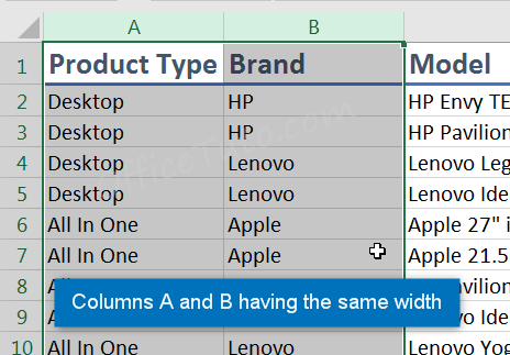
In the following example, I’m applying the same width to columns A and B using the drag and drop of the mouse:

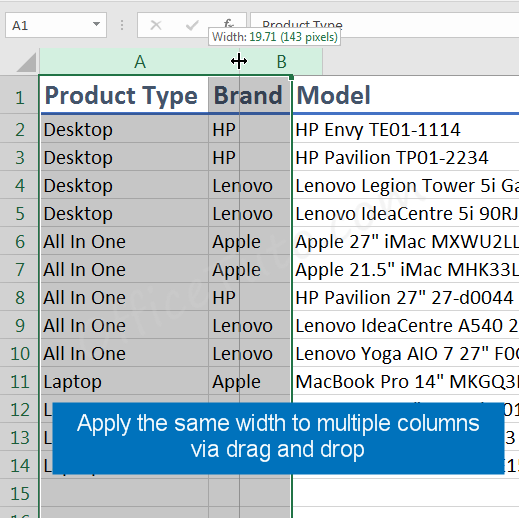
The result is illustrated below:

b- How to make Excel columns the same width via the dialog box

You can set precisely the same width to multiple Excel columns via the “Column Width” dialog box, using the right click or the ribbon.

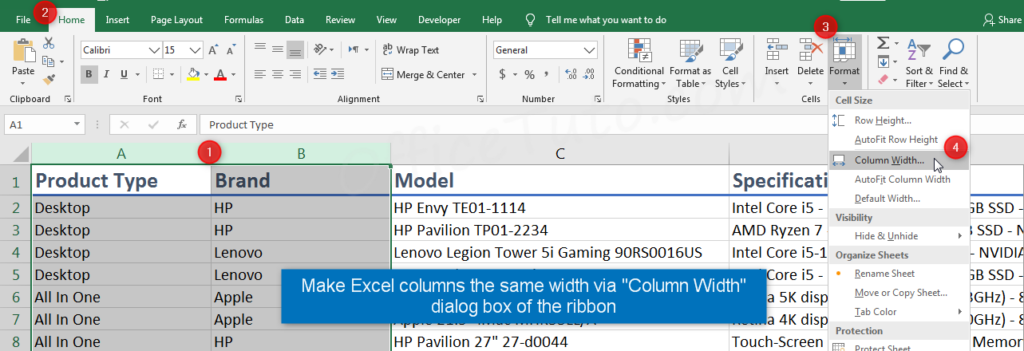
So, to set precisely the same width to multiple Excel columns using the ribbon:

1. Select the columns by their headings.
2. Go to the “Cells” group of the “Home” tab.
3. Click “Column Width” in the “Format” drop-down.
4. Excel displays the “Column Width” dialog box.
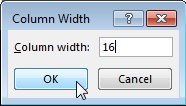
5. Set precisely the column width you want.
6. Click OK to apply the new width to all columns.

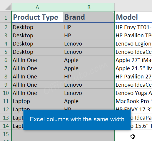
The result of making the same width to columns A and B is illustrated below:

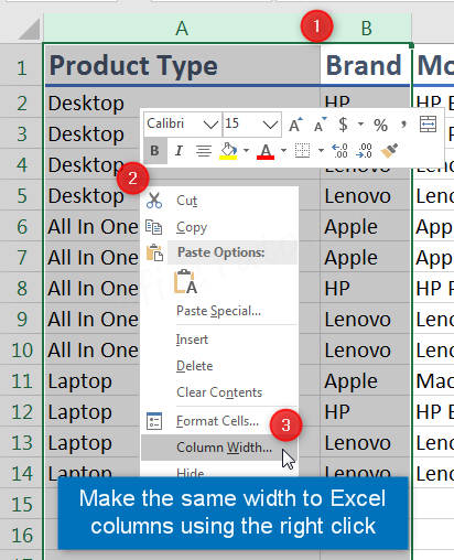
To set precisely the same width to multiple Excel columns using the right click:

1. Select the columns by their headings.
2. Right-click on the selection.
3. Choose “Column Width” from the contextual menu.
4. Excel displays the “Column Width” dialog box.
5. Set precisely the column width you want.
6. Click OK to apply the new width to all columns.

Note: The actual number of characters displayed within the width of the columns (in one line) depends of course on the font, size and style used.

2- How to make Excel rows the same height

Note: I will show you here how to make multiple rows the same height, in one time; this is different than taking the height of one or multiple rows, then applying it in a second time to another ones; for this, you can check How To Copy Columns Width and Rows Height in Excel.

a- How to make Excel rows the same height via drag and drop

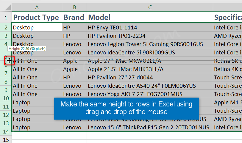
To set the same height to multiple rows in Excel using the drag and drop of the mouse:

1. Select these rows by their headings.
2. Place the cursor on a boundary of any heading of these rows.
3. The cursor is transformed to a double-sided arrow.
4. Click and drag this boundary to the bottom to widen the rows, or to the top to narrow them.
5. All selected rows will take the same size you set.

b- How to make Excel rows the same height via the dialog box

You can set precisely the same height to multiple Excel rows via the dialog box, using the right click or the ribbon.

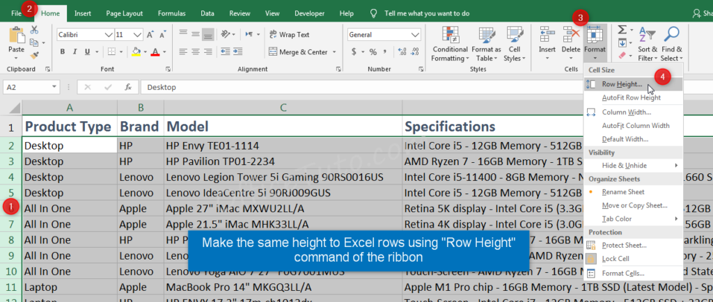
So, to set precisely the same height to multiple Excel rows using the ribbon:

1. Select these rows by their headings.
2. Go to the “Cells” group of the “Home” tab.
3. Click in the “Format” drop-down on “Row Height”.
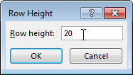
4. Excel displays the “Row Height” dialog box.
5. Set how many points you want as a row height.
6. Click OK.
7. The new height is applied to all selected rows.

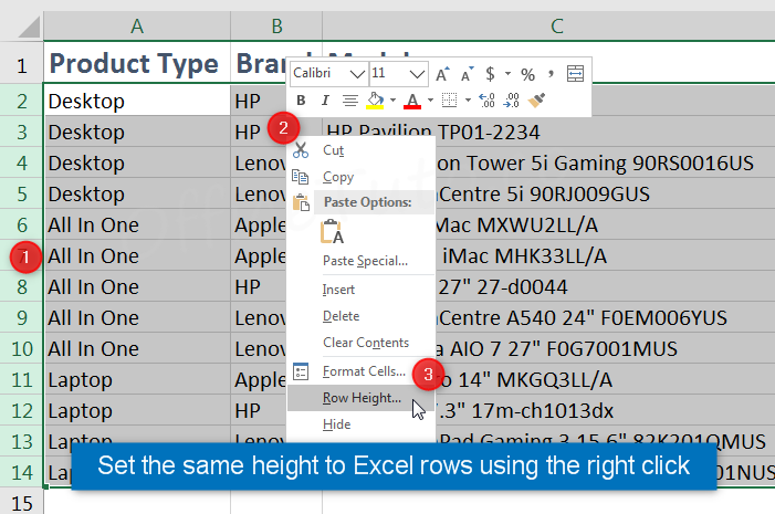
To set precisely the same height to multiple Excel rows using the right click:

1. Select these rows by their headings.
2. Right-click on the selection.
3. Choose “Row Height” from the contextual menu.
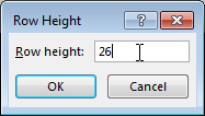
4. Excel displays the “Row Height” dialog box.
5. Set how many points you want as a row height.
6. Click OK.
7. The new height is applied to all selected rows.

G/ Wrap up

That’s all for this tutorial where I showed you how to know the current column width or row height in Excel, what are the minimum and maximum sizes of a cell, how to resize a column or a row, and how to make multiple columns or rows the same size. I also discussed the problem that is sometimes caused by the autofit feature of Excel compared to the manual resizing, and how to correct it.

- "Learn Excel: For Beginners" Series Navigation:

<< 2: Cell Format Types in Excel and How To Implement Them4: How To Copy Columns Width and Rows Height in Excel >>