How to Freeze Rows and Columns in Excel

In this Excel tutorial, we’ll see why and how to freeze a row in Excel, how to freeze a column in Excel, how to freeze multiple rows and columns, and of course how to unlock frozen rows and columns if we don’t need anymore the locked display of information.

A/ Why to freeze rows or columns in Excel

Oftentimes, Excel spreadsheets contain more information than can be displayed on a standard computer screen. Scrolling to data off-screen is easy enough to do, either by using the arrow keys on the keyboard or the on-screen scroll bars.

Scrolling in this way might mean losing visibility of column and row headers needed to understand the information being presented.

To resolve this issue, you have the option to freeze rows and columns in Excel so they persist on screen even when the spreadsheet is scrolled away from those rows or columns, as shown in the following screenshot.

B/ How to Freeze a row in Excel

In the above example, Row 1 on the spreadsheet contains row headers. The information displayed in subsequent rows cannot be clearly understood without seeing these row headers.

I may better lock this top row so it shows all the time even after scrolling.

So, to freeze a row in Excel:

1. Scroll to make the row to lock at the top.
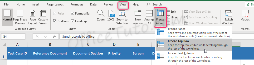
2. In Excel ribbon, navigate to the “View” tab.
3. In the “Window” group, click on “Freeze Panes”
4. Then, choose the option “Freeze Top Row”.

Note: In the first step, when I say “Scroll to make the row to lock at the top”, I literally mean to scroll until the row you want to lock is displayed at the top of the screen right below the column headings (A, B, C…), so Excel can recognize it as the top row of the shown screen. This does not mean, of course, that your row should be placed as row 1 of the Excel sheet; no, it can be any row, you just need to show it at the top by using the vertical scroll bar.

So, if this is not the case, scroll up or down your sheet (depending on your case) until the row you want to lock is shown at the top of the screen (immediately below the column headings).

In my case, the row I want to lock is the headers row (row 1); but keep in mind that, as I said, it can be any row.

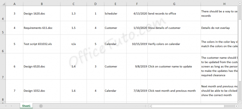
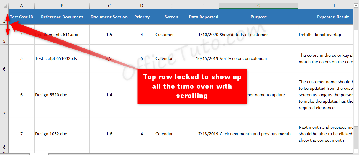
The top row of the spreadsheet will now display even if I scroll down.

Note, in the below screenshot, you see Excel Row 1 and the next row showing is Row 5. This is because Row 1 is frozen and I scrolled down to row 5.

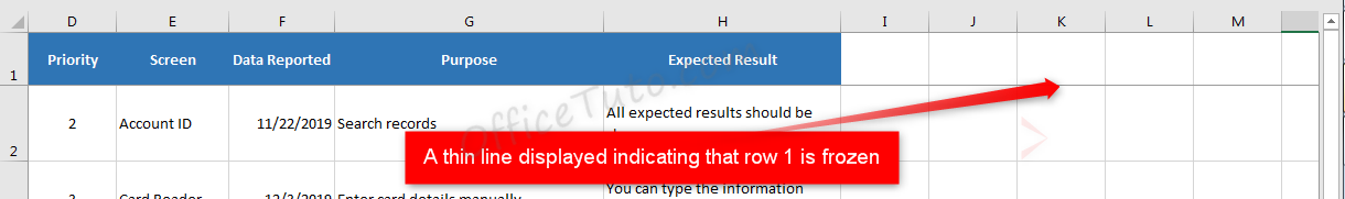
Note also that when you apply the freezing feature on a row, column, or multiple rows and columns, Excel displays a thin line to indicate which part of the spreadsheet is frozen. See the following screenshot from our example of freezing top row.

It may seem repetitive (sorry if it is!), but I would like to emphasize once again that the top row here for Excel is not particularly row 1; it’s just the row you specify as “top row”, the row showed at the top of the screen, when applying the “Freeze Panes” commands.
In other words, you can lock any row you want from your spreadsheet; but, nothing will show above it! If you want the rows above it to show, you can use the other feature of freezing multiple rows; see the following section.

C/ How to freeze multiple rows in Excel

You can freeze multiple rows in Excel instead of a single row as shown right above.

Freezing multiple rows means you will have them all the time displayed regardless of how far you scroll down.

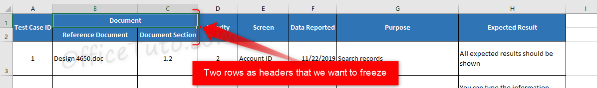
Let’s take our same example as above and suppose I have 2 rows as headers that I need to keep displayed while scrolling down. I added a new row to contain the new “Document” title in B1:C1, and merged the other cells of rows 1 and 2; see the screenshot below.

In our case, I want to freeze the first top rows (row 1 and 2) that have titles of our columns.

So, to freeze multiple rows in Excel:

1. Select the row just below the rows to freeze.
2. Go to the “View” tab of the ribbon.
3. In the “Window” group, click on “Freeze Panes”
4. And choose the option “Freeze Panes”.

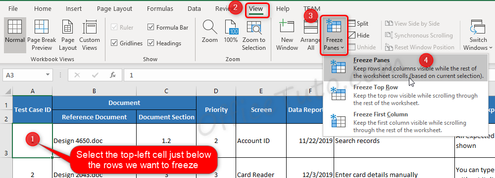
Note that you can, in the first step, either select the row just below the rows you want to lock, or just select the cell to the top-left below them.

In our case, I’ll need to select, at step 1, the row 3 or just the cell A3.

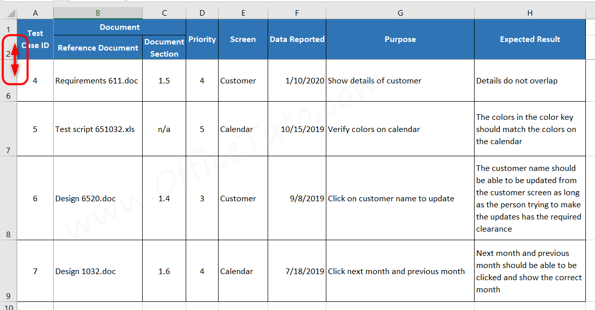
So, after these steps, Excel immediately locks the two rows (rows 1 and 2) as you can see in the screenshot below where I have scrolled down my spreadsheet, and it displays a thin line to indicate that.

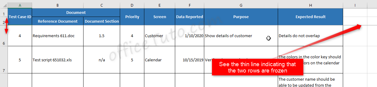
Note that, because row 2 is frozen as long with row 1, when I scroll down to row 6, I find that this row is displayed immediately below row 2.

Tip: which part to select before freezing multiple rows in Excel?!
Just get in mind that when you use the “Freeze Panes” command, Excel always locks what is above your selection and what is left to it.
So, to freeze multiple rows in Excel, you’ll simply need to select the row right below the range you want to freeze, or just the top-left cell below it.

D/ How to Freeze a column in Excel

You may need to freeze a column in Excel when you have data organized in rows and/or have useful headers or titles by rows.

Using the same example as above, I may instead want to ensure that the “Test Case ID” in Column A always displays, even when I scroll to the right to see the information in later columns.

Hence, I would need to freeze column A of our range of data.

So, to freeze a column in Excel:

1. Scroll to make the column to lock at the left.
2. In Excel ribbon, navigate to the “View” tab.
3. In the “Window” group, click on “Freeze Panes”
4. Then, choose “Freeze First Column”.

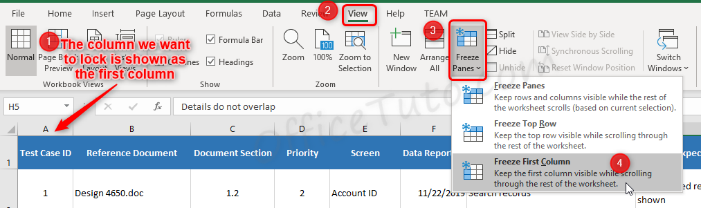
In the first step, when I say “Scroll to make the column to lock at the left”, I mean, If this is not the case, to scroll the horizontal scroll bar until the column you want to lock is shown as the first column of the shown screen (immediately on the right of the rows headings); so Excel can recognize it as the first column of the shown screen.

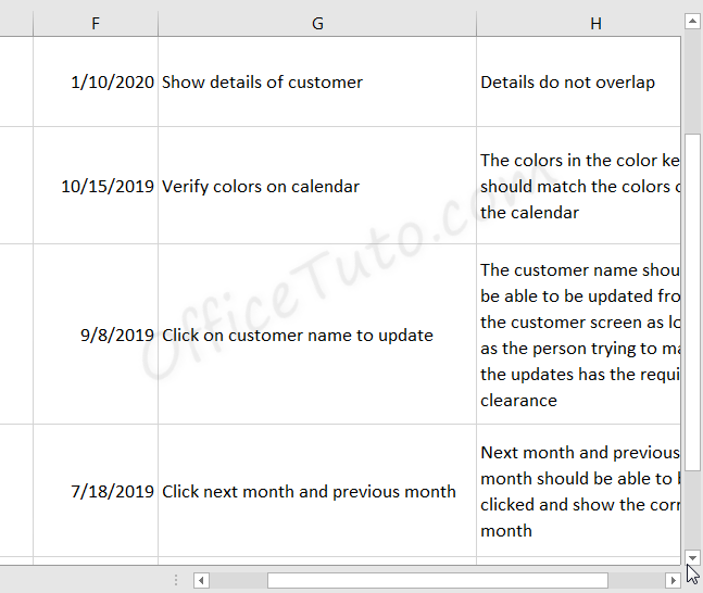
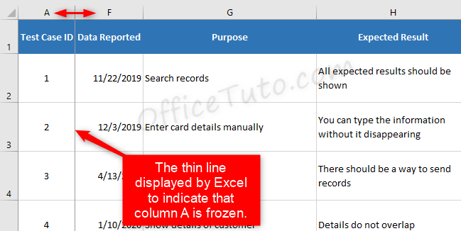
The first column of the shown screen will now permanently display even if I scroll far right.

Note in the below screenshot we see Column A and the next column showing is Column F; this is because Column A is frozen.

Note also the thin line that Excel displays to indicate which column is frozen.

E/ How to freeze multiple columns in Excel

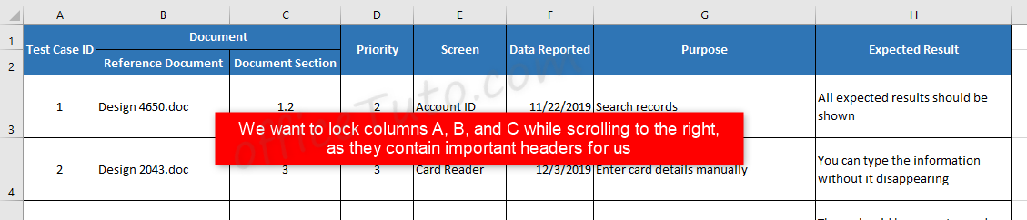
Sometimes, you’ll need to freeze multiple columns in Excel instead of just one column, particularly when you have useful rows headers in more than one column that you want to keep displayed while scrolling to the right of your spreadsheet.

In our case, I want to lock columns A, B, and C while scrolling to the right, as they contain important headers for us.

So, to freeze multiple columns in Excel:

1. Select the column right of columns to freeze
2. Go to the “View” tab of the ribbon.
3. In the “Window” group, click on “Freeze Panes”
4. And choose the option “Freeze Panes”.

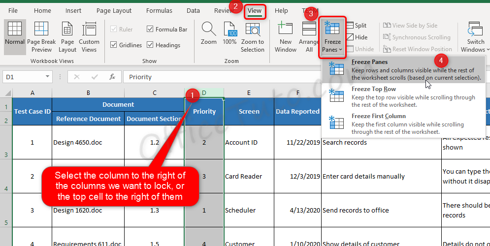
Note that you can, in step 1, either select the column just to the right of the columns you want to lock, or just select the top cell to the right of them.

In our case, I’ll need to select, at step 1, the column D or just the cell D1.

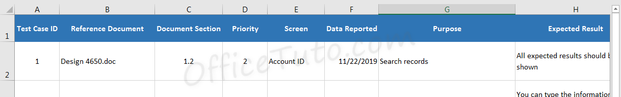
After these steps, Excel immediately locks the three columns (Columns A, B, and C) as you can notice from the screenshot below where I have scrolled right our spreadsheet to column G, and it displays a thin line to indicate which columns are frozen.

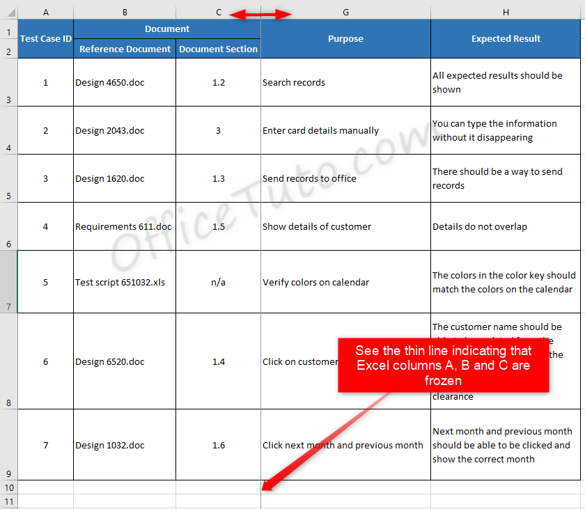
Note also that, because column C is frozen as long with columns B and A, when I scroll right to column G, I find that this column is displayed immediately to the right of column C.

Tip: which part to select before freezing multiple columns in Excel?
When you use the “Freeze Panes” command, Excel always locks what is about your selection and what is left to it.
So, to freeze multiple columns in Excel, you’ll simply need to select the column right to the range you want to freeze, or just the top cell to the right of it.

F/ Freeze rows AND columns in Excel, at the same time

Using the same example I have been working with, I may decide it’s useful to see not only the first two rows containing column headings, but also the first column containing an important ID number I might use to refer to information while presenting it on screen, as well as the listed reference document name in column B and the document section in column C.

So, in summary: I want to freeze both rows 1 and 2, and columns A, B and C!

To freeze both multiple rows and columns in Excel:

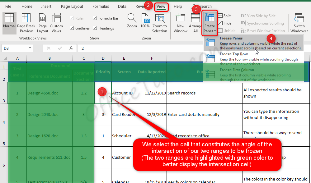
1- Select the top left cell below the rows and right of the columns to freeze; that’s because when using the “Freeze Panes” command, Excel always freezes the ranges above and left to the selected area.

Yes, I know; an example is worth thousand words!

In our example, since I want to freeze rows 1 and 2, and columns A, B and C, the top left cell that constitutes the angle of the intersection of our two ranges is the cell D3; see the screenshot below where I illustrated the two ranges with green color to highlight the intersection cell to be selected.

2- Then, in the ribbon, navigate to the “View” tab and click on the “Freeze Panes” drop-down list in the “Window” group of commands; finally, click on “Freeze Panes”.

Applying these steps, Excel immediately locks the rows 1 and 2, as well as the columns A, B and C.

You’ll notice the thin lines added by Excel to highlight the locked ranges (see the screenshot below).

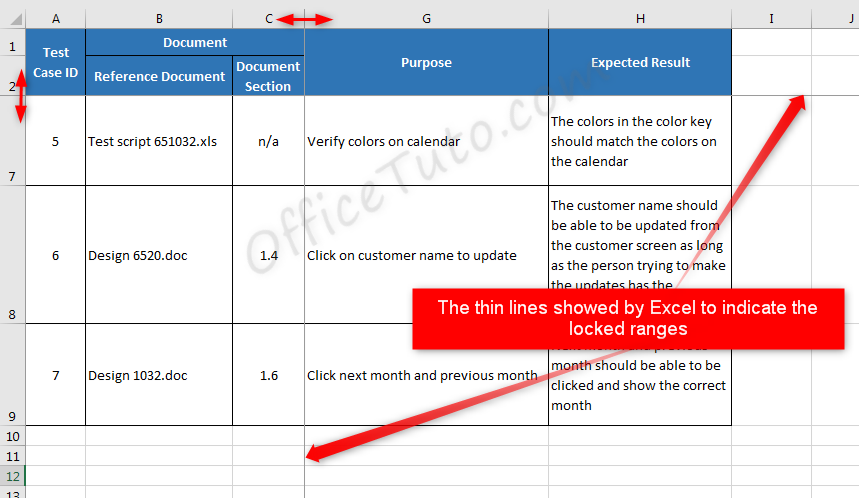
I can now scroll down and right and the information I deemed as pertinent will remain on the screen at all times. In the above screenshot, note Columns A, B and C display, yet the next column shown is G. Additionally, Rows 1 and 2 display, yet the next row shown is 7.

G/ How to unlock frozen rows and columns in Excel

To unlock frozen rows or columns in Excel, just go to the “View” tab of the ribbon, and in the “Window” group of commands, click on the drop-down list “Freeze Panes”; then select “Unfreeze Panes”.

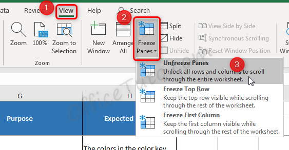
All frozen panes will be unlocked and the spreadsheet will now scroll in the normal way.

---

OK; that was the tutorial on how to freeze rows and columns in Excel.

If you tried this functionality, I’ll be glad to have your feedback in the comments: Did it work well for you, or unfortunately, you encountered an issue implementing it?!

- "Learn Excel: For Beginners" Series Navigation:

<< 7: How to Sort Data in Excel9: How to Filter Data in Excel >>