How to Use Excel: Beginners Guide to Learn All Excel Basics

This tutorial is an Excel tutorial for beginners covering all the basic and common features of this software. It’s an introduction to Excel that will enable you to master Excel basics, quickly and efficiently.

If you follow this tutorial step by step and apply all the instructions detailed here, I can assure you that you will no longer remain a beginner in Excel.

In this Excel tutorial for beginners, I will use versions Excel 2016, 2019, and Excel for Office 365, but the commands and features are quite similar to other versions.

Some guidelines for this tutorial:

• Get in mind that this Excel tutorial will be a very long one; So, to really make the most of it, apply each step in parallel as you read.
• Bookmark this page in your browser, so you can benefit from it in the future.

1- What is Excel

Excel is a software product developed by Microsoft. It is a spreadsheet application, as well as a visualization and analysis tool.

Excel allows the user to create a workbook (the Excel file), in order to store tabular data, perform calculations using Excel formulas, sort or filter data, create charts, etc.

2- Excel Interface

Note: If you didn’t yet open Excel, do it now and create a workbook for the purpose of this tutorial: Launch Excel and, in the welcome screen, click on “Blank workbook”.

Now, keep reading while having an eye on your opened excel workbook.

Once your workbook has been created, the screen will display a main window with a grid to enter information.

I will talk in detail about the elements of this window in the following:

A workbook is the Excel file; it is composed of sheets or spreadsheets.

A spreadsheet is a tabular file where the workspace is organized in rows and columns, and that can contain various data types, such as numbers, text, graphs, etc.

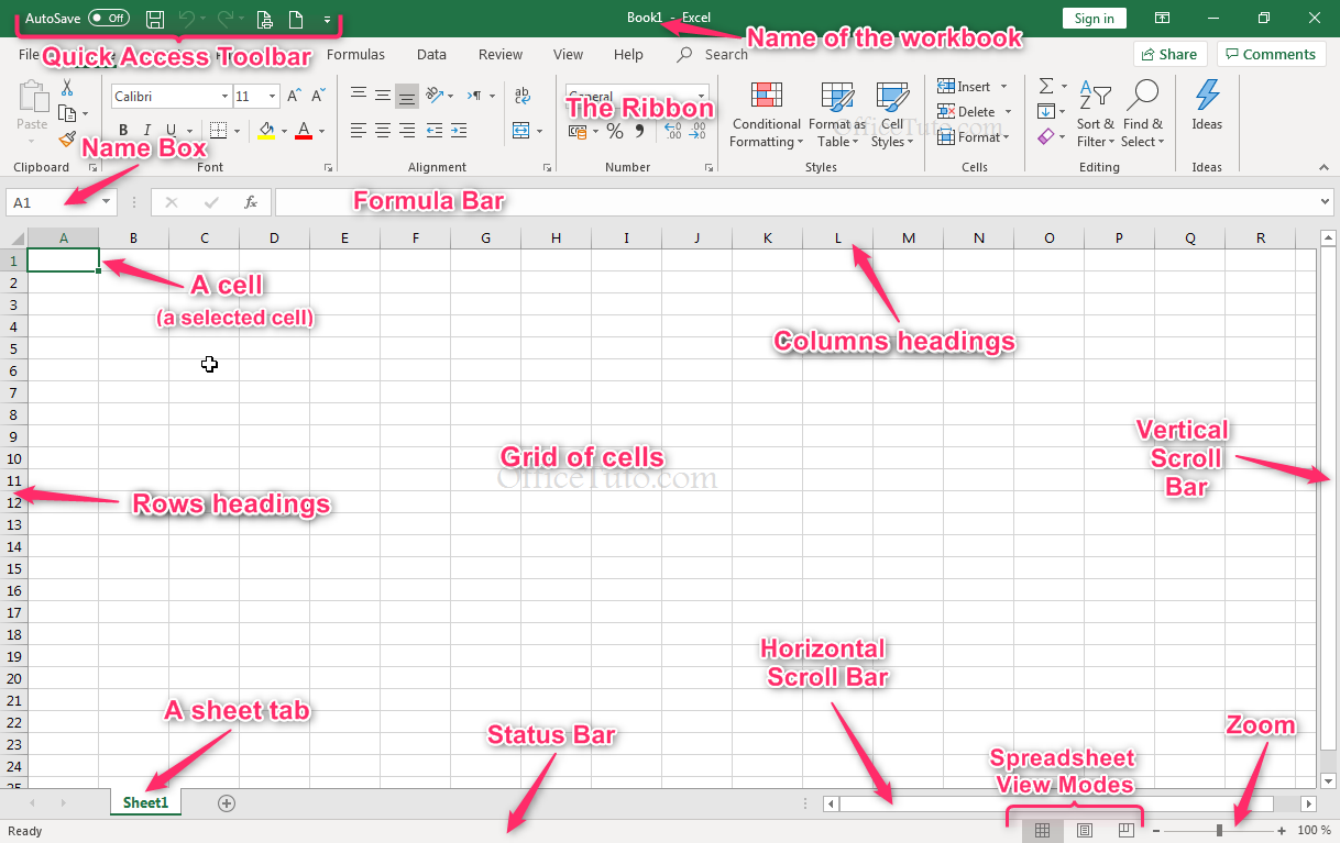
As you can see from the image above that illustrates Excel interface, the intersections of the rows and columns of a spreadsheet constitute a grid of cells, in which information can be entered. The user can enter information in as many cells as necessary from left to right and from top to bottom. The user can then ask Excel to perform calculations such as addition, multiplication, average, etc.

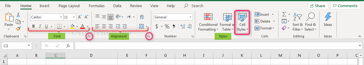
At the top of the Excel workspace, there is the horizontal Excel ribbon that is organized in tabs and that provides all the commands the user needs.

You can use the scroll bars to horizontally or vertically scroll over your spreadsheet.

Above the columns headers, you’ll find the name box that displays the reference of the selected cell, and the formula bar that allows you to enter, edit, and view a formula.

At the top left side, in the title bar, you’ll find the quick access toolbar that provides you with some useful commands that you might use frequently.

And, at the bottom right side, you’ll find the spreadsheet view modes and the zoom tool.

In the following section, I will present the most important elements of an Excel workbook.

3- Description of the elements of Excel workbook and sheet

An Excel workbook is the Excel file; it contains the spreadsheets where you will do all your tasks within Excel.

In the following, I will describe you what are Excel sheets, columns and rows, the cells and references, the formula bar, the ribbon with all its tabs, and the quick access toolbar.

a- Excel sheets

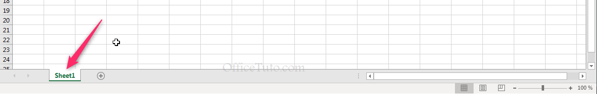
One file (workbook) in Excel can contain one or more spreadsheets, or “sheets”. Sheets are the housing for all the data information which will be contained within them.

Depending on your version of Excel, a new workbook will default to either one or three sheets. This information can be seen at the bottom of the Excel screen.

Different sheets in a workbook are used ideally when separate sets of data are stored.

For example, one sheet might contain a list of all customers for a business and the information about each customer. A second sheet might contain a list of all products sold by the business and information about each of those products. While the information might be related, it is likely separated information being stored about each customer versus each product.

Or, you can use different sheets for different years; etc.

b- Excel columns and rows

A sheet in Excel is organized in Columns and Rows. Columns are of course vertical and rows are horizontal.

By default, columns headings are labeled with letters, and rows headings are labeled with numbers.

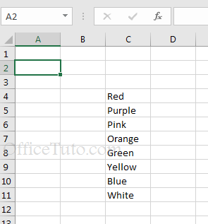
• The below example shows information stored in column C:

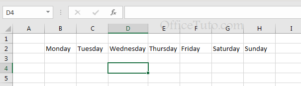
• The below example shows information stored in row 2:

c- Excel cells, their types and references

c1- What is an Excel cell

A cell is one of the rectangles within the sheet. It is the result of the intersection of a row and a column. It is in the excel cells that you will enter your data.

By default, a cell is outlined in a gray color, which means there wouldn’t be any outline at all if the document were printed unless I apply borders to it (more on that later in section 8-e “How to apply borders to Excel cells”).

c2- Data types in Excel cells

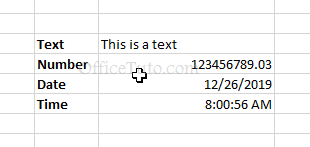
Excel formats cells depending on what type of information they contain: Text, Number, Dates…

By default, a text is aligned to the left and a number is aligned to the right; see the illustration below.

You will find more insights on cell formats in the tutorial: Cell Format Types in Excel.

c3- Cells content and references

• How to enter a content in a Cell:

You can enter a content in a cell, view it, and edit it by clicking directly within the cell itself, but you can also do that in the “Formula Bar” (see the illustration in the following paragraph “Reference of a cell or a range of cells”).

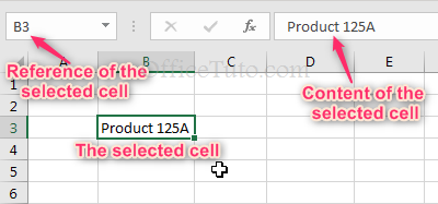
• Reference of a cell or a range of cells:

A cell in Excel is referenced by its column and row.

In the example illustrated below, I selected the cell intersecting column B and row 3. So, the reference of my cell is B3; you can view it in the “Name box“.

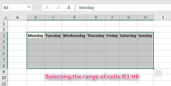
A range of cells is referenced by its first and last cell references, with a colon between them.

For example, I am selecting the range of cells B3:H8 in the following illustration.

References can be used by us to generally refer to cells and ranges of cells, but they are specifically important and essential in Excel formulas.

More on that later in the formulas section of this Excel tutorial.

d- The Formula Bar

The Formula Bar is the bar displayed right above the columns headings.

It is an alternative place of the selected cell where you can enter the content, view it and edit it, and all the changes occurring in the selected cell are synchronously displayed in this bar, as you can notice from the following illustration.

Note that even though it is called the Formula Bar, it can contain every type of content; not just Excel formulas.
The reason for calling it the “Formula Bar” is just because when a formula is entered in a cell, this bar shows the formula itself, not the result as in the cell.

• How to expand and collapse the Formula Bar

The Formula Bar can be expanded to display a larger content, by clicking its arrow. To collapse it, just click again on the same arrow.

e- The ribbon

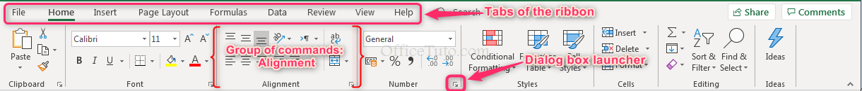
Above the main grid is the navigation ribbon. This ribbon allows quick and easy access to all the options provided by Excel.

It is composed of several tabs that are actually functional groups; that is, they are groups of commands related to some given functions. And, each tab is itself organized in mini-groups of commands with the name of the mini-group displayed at the bottom, and with a dialog box launcher when appropriate.

By default, when a workbook is first opened, the Home tab is displayed.

Below is an outline of some of the basic features of each tab.

e1- Standard tabs of Excel ribbon

Tabs on the default Excel ribbon are:

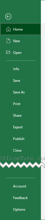
• File (Or “Office Button” for Excel 2007): Contains basic file management options such as create a new workbook, open an existing workbook, save your workbook, print, share (to OneDrive), Export (as a PDf document), and set Excel options.

• Home tab:

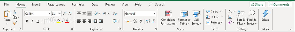
The “Home” tab of Excel ribbon contains some options for commonly used tasks, such as cut/copy/paste, content formatting (font type and size, font style (bold, italic, underlined)), cells borders, cells fill color, font color, alignment of the content of the cells, merge cells, cells formats (number, text, date…), predefined tables and cells styles, insertion and deletion (of sheets, cells, rows, and columns), sort and filter, etc.

• Insert tab:

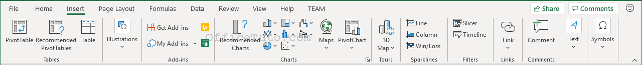
The “Insert” tab of Excel ribbon allows insertion of special Excel elements such as tables, illustrations (pictures and shapes), charts, sparklines (mini-charts), links, comments, special text (text boxes, header and footer, and WordArt), and symbols (mathematical equations and symbols).

• Page Layout tab:

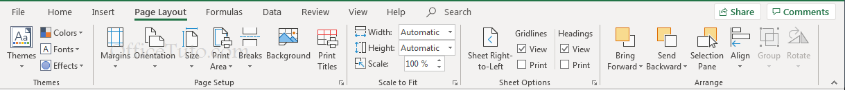
The “Page Layout” tab of Excel ribbon allows themes to be applied to the workbook; provides some options that affect how the pages will display when printed, such as adjusting margins, changing page orientation from portrait to landscape and vice versa, and choosing the rows or columns to repeat on each printed page (titles/headers of your table); some sheet options like setting the sheet to show left to right or right to left, and choosing to view and print gridlines and headings.

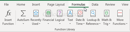
• Formulas tab:

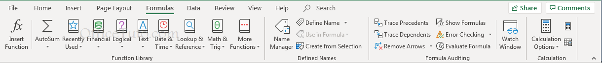
The “Formulas” tab of Excel ribbon provides commands and drop-down menus to create formulas with functions from the vast Excel functions library.

You can insert a function using the “Insert Function” command of this tab, or by choosing from the provided categories (drop-down menus). More on that below in the formulas section of this Excel tutorial.

This “Formulas” tab also allows to define (and manage) a name for a cell or a range of cells. A name of a cell or a range of cells can be used in Excel formulas instead of references.

• Data tab:

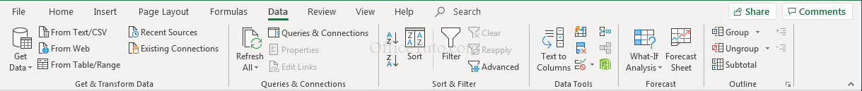
The “Data” tab of Excel ribbon provides some advanced features like options to import data from external sources (like other files (Excel workbooks or others), databases, web, etc), and perform queries of databases.

There are also some other important features like to sort and filter data within the spreadsheet (these are the same options as in the “Home” tab, plus some advanced features), split a column of text in multiple ones following a criteria (fixed width or a special character (like a space, comma, tab, period…)), automatically fill in values using the flash fill feature (following an example entered by the user), remove duplicates, set rules for data that can be entered in a cell, and create an outline by grouping some rows or columns.

• Review tab:

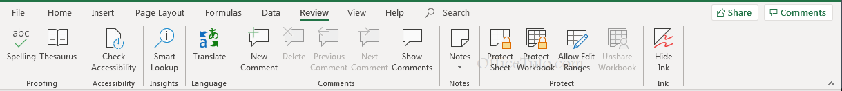
From the “Review” tab of Excel ribbon, you can use the Excel spell checker and thesaurus to check and correct the text content of your spreadsheet; you can translate your text to another language, create and edit comments or notes, and protect (lock) elements of the workbook.

• View tab:

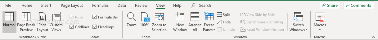
The “View” tab of Excel ribbon gives you options to change the on-screen display of your sheet (Normal view, Page Break, Page Layout, or Custom view); show and hide the gridlines, the formula bar, and the headings of the rows and columns of your sheet; apply a zoom; freeze panes (useful to keep the headers of your tables visible while you scroll over your spreadsheet); view 2 sheets side by side (to, for example, compare their content); and create macros.

• Help tab:

The “Help” tab of Excel ribbon shows links to Excel software help documentation and to Microsoft Online training.

e2- Contextual tabs of Excel ribbon

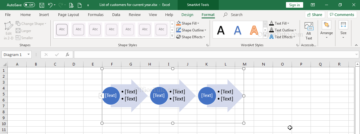
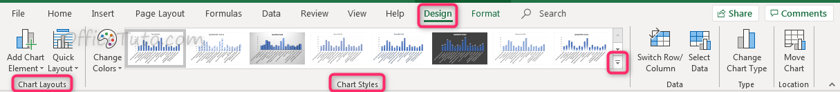
Other tabs may display on the ribbon depending on what you are working on within the Excel sheet. They include the following tabs: Draw, Developer, Design, Format, Analyze, Pens, and Query.

As an example, here are the contextual tabs that display when selecting a SmartArt graphic: “Design” and “Format” tabs (see the following screenshot).

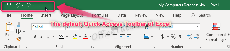
f- Quick Access Toolbar

The Quick Access Toolbar is the toolbar that stands on the top-left side of your Excel window.

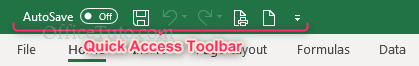
Its purpose is to provide very quick and easy access to the most used commands.

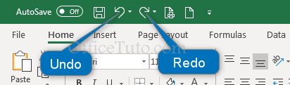
By default, it stands on the top-left side and displays only 3 buttons: Save, Undo, and Redo.

But, you can customize its placement and the buttons showed in. More on that in section 16 of this Excel tutorial.

4- How to create and save a Workbook

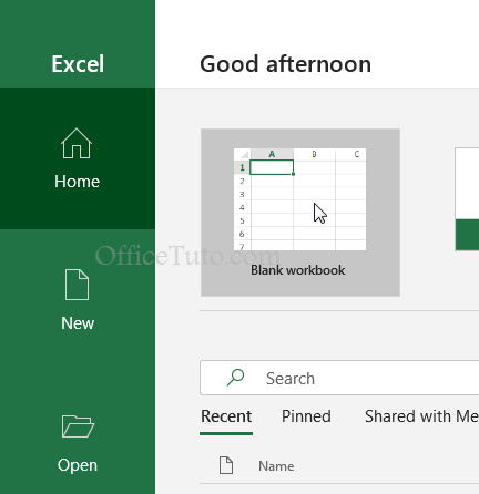
When you first launch Excel, the main screen (which may look different depending on your version of Excel) will offer the option to create a Blank workbook. This is an Excel file (workbook) without any data already in it. Click on “Blank workbook”.

You’ll get a screen similar to the image from section 2.

It is always a smart idea to save your work, even before you’ve gotten started.

To save, go to File (or “Office Button” for Excel 2007) → Save As, or File (“Office Button” for Excel 2007) → Save.

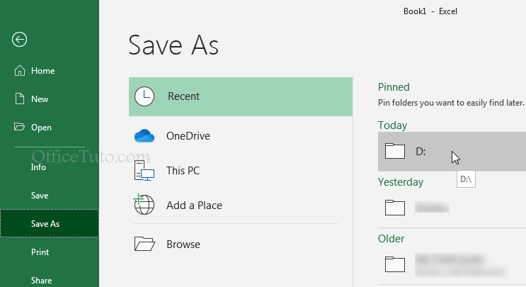
The options presented on the “Save as” screen offer various locations you can save to. You can choose recent locations from the right panel when the “Recent” option is selected, or you can choose another location like OneDrive, or any folder from your computer by selecting “This PC” or “Browse”.

In my case, I chose to save the file to the D partition from my recent locations.

Once a folder is selected to save to, Excel prompts us to enter a filename. Enter a name that is descriptive about the file being created.

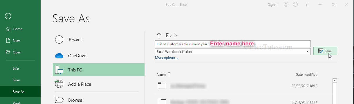
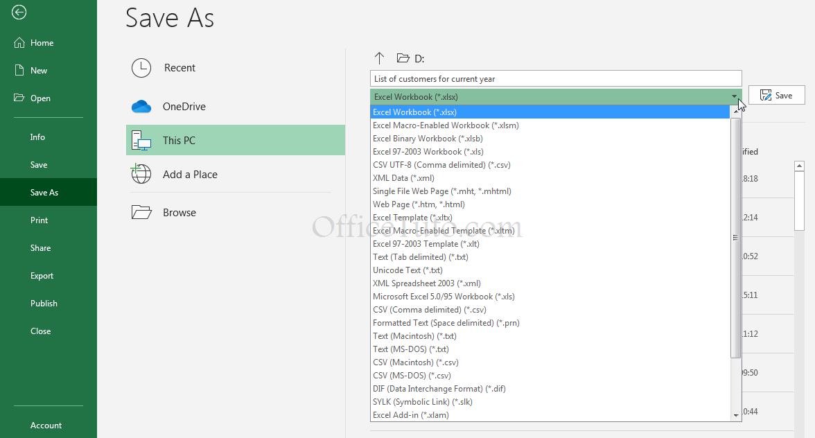
Note that the second field shows the type of file being creating – an Excel workbook.

New versions of Excel (starting from version 2007) create workbooks with a file extension of .xlsx. The drop-down of this second field offers a large selection of other file extensions which the workbook can be saved as. This would be useful for saving a file in a format which could be read by people who have an older version of Excel (extension .xls), to save as a simple Comma Separated Values file (extension .csv) which can be read by many sources, or for many other reasons depending on the file’s intended use.

For this example, the normal .xlsx extension will be used. Click Save to continue back to the blank workbook which has now been created and saved.

5- How to manage sheets in an Excel workbook

Excel sheets can be added, renamed, copied, moved, reordered, tab colored, hidden, protected, and deleted.

a- How to add a new sheet in an Excel workbook

To insert a new sheet in your Excel workbook, you have three ways:

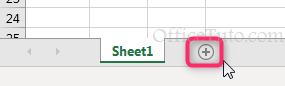
a1- Add a new sheet using the New sheet button

This first method is the easiest one: Click on the “New sheet” button, at the bottom of the screen next to the sheets tabs; a new sheet is immediately inserted in the workbook.

a2- Add a new sheet using the right-click button of the mouse

Right-click on a sheet name → This will bring up a pop-up menu (see the screenshot below): Click on “Insert” → The “Insert dialog box” shows up; check that “Worksheet” is selected, then click on OK.

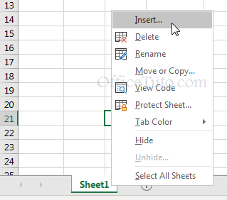
A new sheet is then added to the existing ones of your workbook.

a3- Add a new sheet using the ribbon

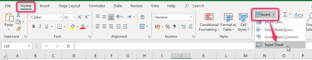
Go to the “Home” tab of Excel ribbon → In the group of commands “Cells”, click on “Insert“, then “Insert Sheet“.

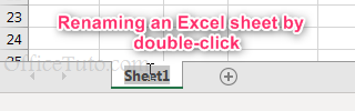
b- How to rename an Excel spreadsheet

By default, Excel names the sheets Sheet1, Sheet2, Sheet3, etc.

But, you can rename an Excel sheet as you like, to reflect better its content. Here is how to do:

Just double-click on the sheet’s name in its tab; Excel will highlight this name → Then, type the name you want for it.

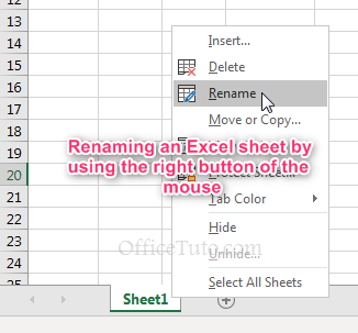
You can also use the right button of the mouse for that:

Just right-click on the sheet’s tab and select “Rename“. Excel will highlight the name to allow you to edit it.

c- How to copy an Excel spreadsheet

You may need to copy an Excel sheet to the same workbook or to another one, to create a new sheet with the same structure or similar as the current one; for example, to create another sheet for a different period of time (another year, month, or whatever), or for another client or product…

Anyway; this is how you need to proceed:

c1- How to copy an Excel sheet to another workbook

My source file is the “List of customers 2019” workbook that contains the sheet “Q1”, and I want to copy this sheet to another workbook to work on it.

First, if the target workbook already exists, you should open it; otherwise, if you want to copy your sheet to a new workbook, do nothing.

In my case, I want to copy the sheet to a newly created workbook; so, I don’t have to open any other workbook or to create this new one; Excel, as we will see in the following, will do it automatically during the process.

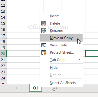
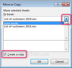
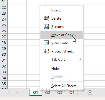
Now, get back to the source workbook (from where I want to copy. In my example, it’s the “List of customers 2019” workbook) → Right-click on the tab of the sheet you want to copy (See the screenshot below) → Click on “Move or Copy“.

The “Move or Copy” dialog box shows up (See the following screenshot) → Always begin by checking the “Create a copy” checkbox, so Excel copies the sheet rather than moving it → Then, click the arrow of the “To book” drop-down list to choose the target workbook where I will paste my copied sheet. In my example, I chose the “new book” option, so that Excel creates for me a new workbook and placed my sheet in it → Click “OK” of course.

Excel then opens the target workbook (an existing or a newly created one) with the sheet (a copy of my source one) in it. It will call it “Book2”; so, you need to save it where you want, with a name you choose.

Note: In my example, as you may notice, there isn’t any other workbook listed in the “Move or Copy” dialog box, other than my source workbook “List of customers 2019”. And that’s because I didn’t open another existing workbook since I had the intention to copy my sheet to a newly created workbook.

c2- How to copy an Excel sheet in the same workbook

• Copy an Excel sheet in the same workbook using the Right-Click method

To copy an Excel sheet to the same workbook, you can follow the same steps as in the previous section c1, using the “Right-Click” method; meaning:

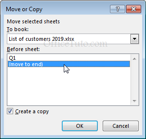
Right-click on the tab of the source sheet (the spreadsheet you want to copy) → Click on “Move or Copy” → Excel displays the “Move or Copy” dialog box where you have to  check the “Create a copy” checkbox (to copy the sheet rather than move it) → Here, you don’t need to click the arrow of the “To book” drop-down list to choose the target workbook which needs to be the same source workbook, as Excel selects by default the source workbook in it. But, you may need to choose the position of your new sheet in the target workbook (meaning, where to place it exactly within the existant sheets): choose the option you want in the “Before sheet” field. In my example, I chose to place it at the end → Click “OK“.

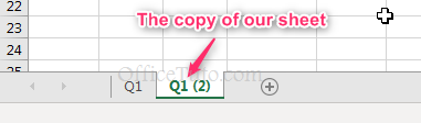
Excel creates a copy of your sheet in the same workbook, with the name “source_name (2)”. In my case, I copied the “Q1” sheet in my same workbook, and Excel called the copy “Q1 (2)”.

You can rename it as you like, as we learned earlier in section 5-b of this Excel tutorial.

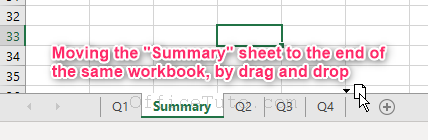
• Copy an Excel sheet in the same workbook using the “Drag and Drop” method

This method is much easier than the previous one as you just use your mouse to drag the tab of the sheet source (you want to copy) where you want in the workbook and drop it as a copy; here is how to do:

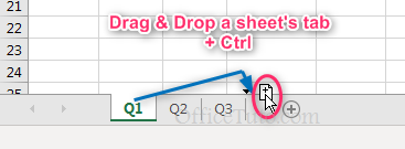
Go to the tab of the sheet source (you want to copy); in my illustrated example, it’s the spreadsheet “Q1” → Click with the left button of the mouse and drag it through the sheets tabs to the placement you want → Without releasing the left button of the mouse, press “Ctrl” key of your keyboard; you’ll notice a plus sign that appears beside the cursor on the sheet’s icon → Then, drop the sheet’s tab by releasing the left button of the mouse, and release Ctrl key→ You’ll get then a copy of your sheet added to your workbook.

d- How to move an Excel spreadsheet

d1- Move an Excel spreadsheet to another workbook

The method of moving an Excel sheet to another workbook is the same as copying it, except for checking the “Create a copy” checkbox. Here, I simply won’t check it!

So, my source file will be again the “List of customers 2019” workbook that contains now the sheets “Q1“, “Q2“, “Q3“, and “Q4“; and I will move the first sheet “Q1” to another workbook, be it an already existing workbook or a newly created one (created automatically by Excel during the process).

If the target workbook already exists, open it; otherwise, if you want your sheet to be moved in a newly created one, do nothing and continue with the following:

In this example, I will move my sheet to an existing workbook, the “List of customers 2020“.

So, I will get back to the source workbook, “List of customers 2019”. To move my sheet, I will right-click on its tab, then choose “Move or Copy” as illustrated below.

Excel displays the “Move or Copy” dialog box, where I will choose the target workbook, as well as the placement of my sheet among the other sheets.

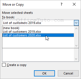
In the “To book” field, I select the target workbook: In my case, it’s the “List of customers 2020” workbook.

[Note: If I choose here the “new book” option as a target, Excel will create a new workbook and place the moved sheet in it].

And in the “Before sheet” field, I select the sheet before it I want to place my moved one, or the “move to end” option if I want to place my sheet at the end of the sheets’ group: In my case, I chose to place it before the first sheet (Sheet1).

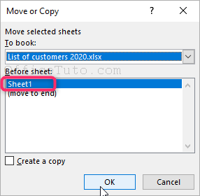
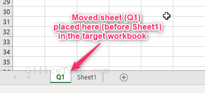
Once I click “OK“, Excel will move my sheet into the new workbook and my source workbook will no longer contain it.

d2- Move an Excel spreadsheet in the same workbook

To move an Excel sheet into the same workbook, you can follow the same steps as moving it to another workbook, as detailed in the previous section “c1”, with the exception of selecting the same workbook in the “To book” field of the “Move or Copy” dialog box.

But, you can do better by choosing a much easier and quicker way, which is the “drag and drop” method:

With this method, you just need to drag the tab of the sheet by pressing the left button of the mouse and, while holding it down, drag it where you want among the existing sheets of the current workbook.

e- How to delete a sheet in an Excel workbook

As for anything material in this world, deleting an Excel sheet is very quick and easy!

And you can do it in two ways:

– Delete an Excel sheet using the ribbon

Be sure that the sheet you want to delete is selected; meaning, it’s the one currently displayed. If not, click on its tab to select it → Then, go to the “Home” tab of the ribbon, and in the group of commands “Cells”, click on “Delete“, then on “Delete Sheet“.

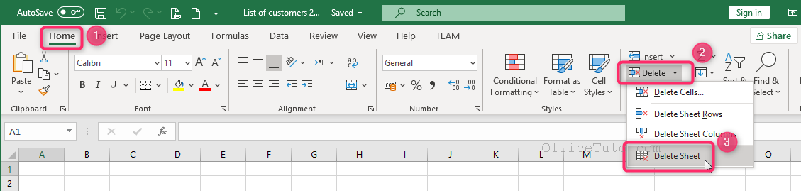
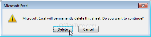
If your sheet contains any data, Excel will show a warning message for you to confirm the deletion. Click “Delete” to confirm.

– Delete an Excel sheet using the right-click menu

Deleting an Excel sheet using the right-click menu is much easier than the first method:

You just need to right-click on the tab of the sheet to be deleted and choose the “Delete” command.

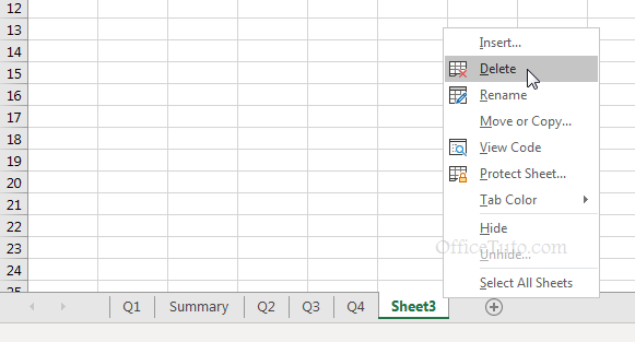
If your sheet has any data on it, Excel will ask for a confirmation from you with a warning message; otherwise, it will directly delete it.

If this occurs, click “Delete” to confirm.

6- How to enter, edit, format and wrap data in a spreadsheet

a- How to enter data in an Excel spreadsheet

It’s very easy to enter data in an Excel sheet; you just select the cell where you want to enter data, by clicking on it, and type in what you want; when you’re done, press Enter to validate your data.

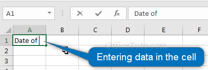
You can also use the “Formula Bar” after selecting the desired cell, and press Enter to validate; but, it’s much easier to directly type in the cell itself.

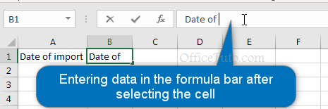
You may find entering data in the “Formula Bar” more useful when there is a lot of data; but, I think it’s just a matter of personal choice, and it’s up to you to choose the way you prefer: entering data directly in the cell itself or via the Formula Bar.

Note: Just keep in mind that, whether you choose to enter data in the cell itself or through the formula bar, the cell and the formula bar will synchronously reflect the same thing (as you can notice from the two previous images).

– Data types/Cells formats:

When you enter any data in a cell, Excel automatically chooses the right format for the cell that better corresponds to its content.

In general, Excel assigns the following formats:

– The format “Date” when you enter a date with any of these formats 12/03/2019, 12/03/19,  12-03-2019, or 12-03-19.

– The format “Currency” when you enter a number with this format $12.35, or $ 12.35.

– The format “Percentage” when you enter a number with this format 12.35%, or 12.35 %.

– The default format “General” for any other numeric and text data.

But, you can decide yourself for the cell’s format in the “Number Format” drop-down list from “Home” tab of the ribbon, if the format automatically assigned by Excel doesn’t fit your needs; see image below:

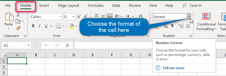
So, to change the format of the selected cell, go to “Home” tab of the ribbon → Click on the “Number Format” drop-down list, and select the format you need.

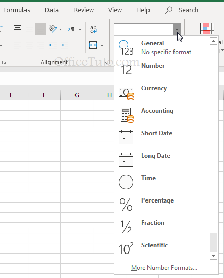
The different formats of cells provided in this drop-down list are:

• General
• Number
• Currency
• Accounting
• Short Date
• Long Date
• Time
• Percentage
• Fraction
• Scientific
• Text
• And the “More Number Formats” option.

Clicking the option “More Number Formats” brings up additional options for formatting cells, including the ability to do special and custom formatting options.

Note: You can update a cell’s format before or after entering data to adjust the way the data appears.
For example, changing the format of a cell to “Currency” will make its content displayed as a dollar amount.

The tutorial Cell Format Types in Excel explains in detail what are cell format types in Excel and how to implement them.

b- How to edit data in Excel

To edit data already entered in an Excel cell, you can follow two methods:

– Edit data in the cell itself

Double-click on the cell you want to edit the content → Place the cursor of the mouse where you want into the content of the cell → Change what you want → Then press Enter.

Note: There is a difference between editing a content in a cell, and completely replacing it.
If you want to just edit it, do as we just learned by double-clicking on the cell; but, if you want to completely replace the content of the cell by a new one, click the cell (not double-click!) and type the new content.

– Edit data using the Formula Bar

Another way to edit a content of a cell is to use the formula bar: Just select the cell you want to edit (by clicking on it) → Go to the “Formula Bar” and edit the content as you want (partially or completely) → Press Enter.

c- How to format data in Excel

All data in Excel cells can be formatted using the formatting features in the “Home” tab of the ribbon, for the content of the selected cell, or for the cell itself.

This includes the font, the style of the font (Regular, Bold, Italic, Underlined…), the size of the content, the font color, the alignment of the content (Horizontal alignment and Vertical alignment), the indentation, the orientation of the content (rotation), and the fill color of the cell (color of the cell’s background); as well as some predefined styles for the cells.

All these features can be accessed from the “Home” tab of the ribbon, in the 3 groups of commands “Font“, “Alignment“, and “Styles“.

Just select the cell or range of cells (or even a whole row, column, or many rows or columns, from their headings) you want to change the formatting, and apply the features you want.

Note: Keep in mind that you can always undo the changes if anything goes wrong, as well as redo them, using the respective commands “Undo” and “Redo” of the Quick Access Toolbar.

d- How to wrap text in a cell

Wrapping text in a cell is making it in multiple lines in the same cell, without inserting a line break; the number of lines the text will display on will depend on the width of the column and the height of the row.

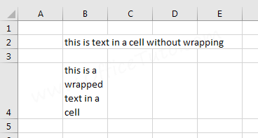
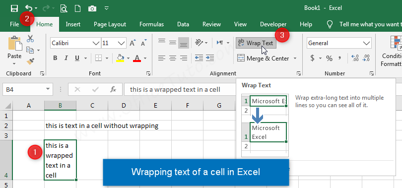
Now, to wrap a text in a cell, just select this cell, then go to the “Home” tab of the ribbon, and in the group of commands “Alignment“, click on the “Wrap Text” command. Excel will restrict the display of the text to the dimensions of the cell: its width and height.

7- How to manage rows and columns in Excel

In Excel, you can insert rows and columns, change their position, change the width of columns and the height of rows, or delete them.

But to do all of these things, you must select your rows or columns, except for changing the widths and heights where the selection step is not all the time necessary.

More on that below.

a- How to select rows or columns in Excel

a1- Select a single row or column in Excel

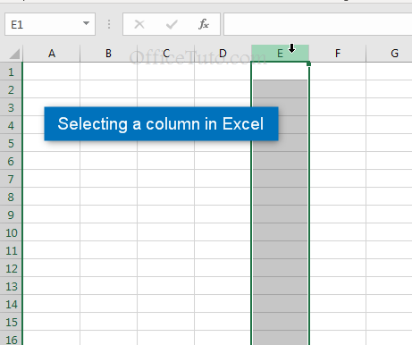
To select a row or a column in an Excel sheet, you just need to click on its heading.

In the screenshot below, I am selecting column E by clicking on its heading.

a2- Select multiple adjacent rows or columns in Excel

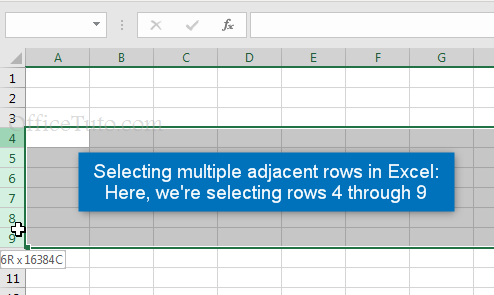
To select many rows or columns that are contiguous, you just need to click on the heading of the first row or column and, while holding down the left button of the mouse, select the others by going through their headings.

Or, you can just click on the heading of the first row or column, hold down the “Shift” key of the keyboard and click on the heading of the last row or column.

In the screenshot below, I am selecting rows 4 through 9.

a3- Select multiple non-adjacent rows or columns in Excel

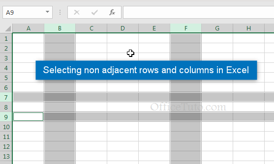
To select non-contiguous rows or columns in Excel, you need to select one row or column (by clicking of course on its heading), hold down the “Ctrl” key of the keyboard and select the other row or column, and so on.

In the screenshot below, I am selecting columns B and F, and rows 7 and 9.

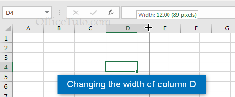
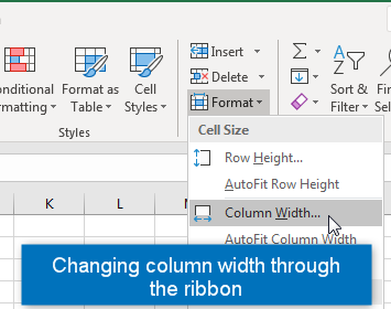
b- How to change column width in Excel

To change the width of a column in Excel, you can simply go to its heading and position the mouse cursor at its border (on the side where you want to expand its size (left or right side)), so that it turns into a double-arrow as you can see from the screenshot below, then drag it to the desired width.

This is my preferred method, but you can do otherwise through these 2 additional methods:

• by using the ribbon:

Select the column → Then go to the “Home” tab of the ribbon → In the “Cells” group of commands, click on “Format“, then on  “Column Width” → A dialog box will show up where you can enter the width you want for your column → Click OK.

• By a right-click on a selected column:

Select the column → Right-click on it anywhere and choose “Column Width” → A dialog box will display to allow you specifying the exact width you want for your column → Click OK.

For more in-depth info and detailed examples on how to change the width of a column in Excel, check How To Change the Columns Width and Rows Height in Excel.

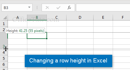
c- How to change row height in Excel

Changing the height of a row in Excel is identical to changing a column width.

Start by going to the row’s heading and position the mouse cursor at its border (on the side where you want to change its height (bottom or top side)), so that it turns into a double-arrow (see the screenshot below), then drag it to the height you want.

Here again, you can use 2 additional methods:

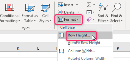
• by using the ribbon:

So, select the row → Next, go to the “Home” tab of the ribbon → And, In the “Cells” group of commands, click on “Format“, then on  “Row Height” → A dialog box will show where you can enter the height you want for your row. Do it, then click OK.

• By a right-click on a selected row:

Select the row → Right-click on it anywhere and choose “Row Height” → A dialog box will show up to allow you specifying the exact height you want for your row→ Click OK.

For more in-depth info and detailed examples on how to change the height of a row in Excel, check How To Change the Columns Width and Rows Height in Excel.

d- How to insert rows and columns in Excel

In an already filled table, you would need to insert new columns and rows.

There are 3 methods: I will show you here the easiest one of them, and will just mention the other two without going deeper (this Excel tutorial is already getting too long and too detailed for beginners).

• 1st method: Right-click on the heading

So, to insert a column or a row in Excel, click with the right button of the mouse on the heading of the row or column, and choose “Insert“.

Excel will insert a new column before the selected column, or a new row above the selected row.

Here is the result of the insertion operation from the screenshot above:

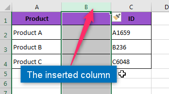
In this example, a new column was inserted by Excel before the selected one (Column C).

• The other 2 methods:

In addition of this 1st method, you can insert a row or column in Excel by right-clicking on a cell from the row or column you want to insert another above or before, respectively; as well as by using the “Insert” drop-down list from “Home” tab of the ribbon.

e- How to delete rows or columns in Excel

Here again, there are 3 ways to perform this task: By right-clicking on the heading, by right-clicking on a cell from the column or row, and by using the ribbon.

• Delete a row or a column by right-clicking on its heading

Right-click on the heading of the row or column you want to delete → Choose “Delete“.

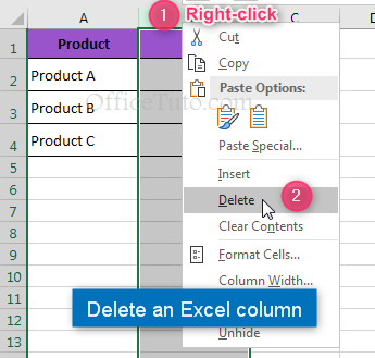
Excel will immediately delete this row or column.

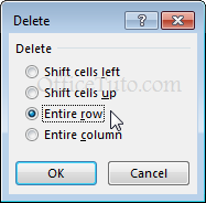
• Delete a row or a column by right-clicking on a cell from it

Right-click on a cell from the row or column you want to remove → Choose “Delete” → In the dialog bow that shows up, select “Entire row” or “Entire column” depending on what you intend to do → Click OK.

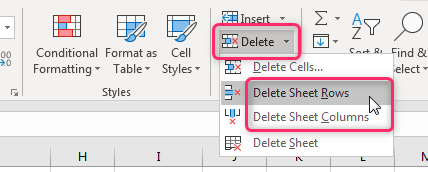
• Delete a row or a column by using the ribbon

Click on a cell from the column or the row you want to remove → Go to the “Home” tab of the ribbon, and in the group of commands “Cells”, click on “Delete“, then choose “Delete Sheet Rows” or “Delete Sheet Columns” depending on what you want.

8- How to manage and format cells in an Excel spreadsheet

I will show you in the following how to insert cells in an Excel spreadsheet, how to merge them, how to move them, how to delete them, how to apply borders to them, and how to color their background.

a- How to insert cells in Excel

I am talking here about inserting cells, not entire rows or columns.

You may need to insert cells into an already populated table where you need to add new items that were not originally planned, but you have another table next to it or below it; so, if you want to add an entire Excel row or column for the new items, you will totally mess up your organized data in the other tables (see the screenshot below).

Therefore, the solution is to insert cells, rather than entire rows or columns; here is how to do:

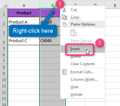
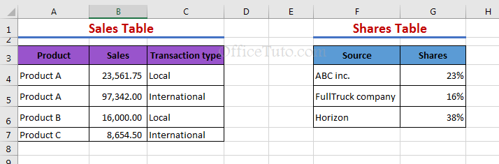
In my example (see the screenshot below), I have 2 tables in the same sheet, one next to the other; and I want to add, in the “Sales Table”, another sale and transaction type for “Product A”, before the second item “Product B”.

Note: The organization of data is not optimal, but I’m deliberately using this example for the purpose of this tutorial.

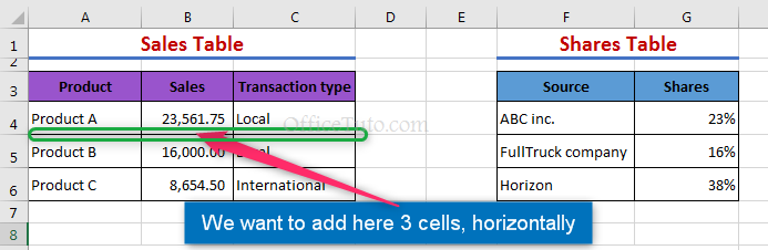
I won’t add an entire row after “Product A” because this will mess up my other table “Shares Table”, and I won’t add just 2 cells in B5 and C5, as this will mess up my current table “Sales Table”; rather, I will add 3 cells under “Product A” row for my new data: one for the product’s name (which is, in this case, the same “Product A”), one for the sales amount, and a last one for the transaction type.

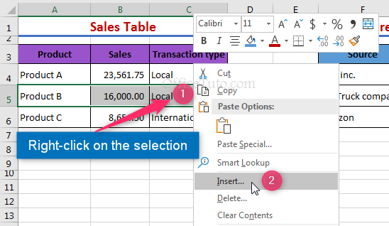
Let’s then select the 3 cells above which I will add my new ones; in this case, the range of cells A5:C5 → Right-click on the selection and click “Insert“.

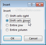
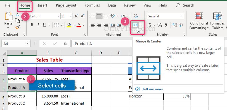
Excel will display the dialog box “Insert” where I will choose the “Shift cells down” option, to shift down the 3 cells of “Product B” and every other cells below them, and make room for the new ones → Then click “OK”.

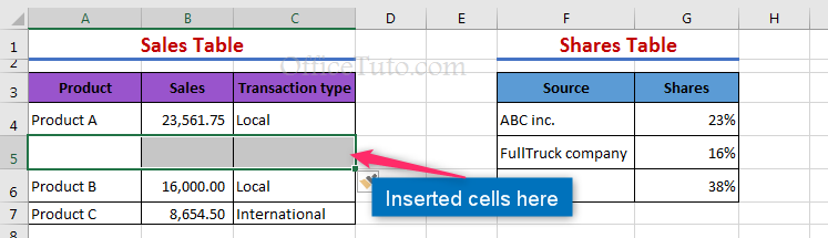
Here is the result:

And after entering the new data:

Inserting new cells in an Excel table may result in some changes in the existing tables on the same sheet, so you may need to perform extra tasks, such as merging cells or moving them.

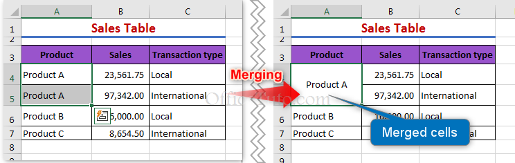
For example, I may want to merge the cells A4 and A5 (from screenshot above) into a single one with “Product A” as its content.

See the following paragraphs.

b- How to merge cells in Excel

– Merge cells in Excel:

You need first to select them, then go to the “Home” tab of the ribbon, and in the groups of commands “Alignment”, click on the “Merge & Center” command.

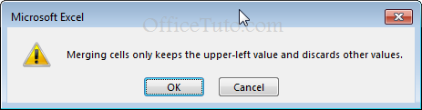
If the upper-left cell and another one(s) contain data, Excel will first warn you by a message that all content will be removed except for the content of the upper-left cell.

Here is the result of merging cells A4 and A5 from my example:

– Unmerge cells in Excel:

To unmerge already merged cells in Excel, you just need to select the merged cells and click the “Merge & Center” command from the group of commands “Alignment” in the “Home” tab of the ribbon.

Yes, the tool “Merge & Center” has a double effect: Merging and Unmerging.

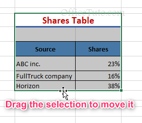
c- How to move cells in Excel

To move cells in Excel, select them, then place the mouse cursor on the border of the selection. It takes the form of a double-arrow (see screenshot below) → Drag the selection where you want.

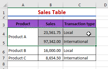
d- How to delete cells in Excel

I am here talking about deleting the cell itself, and not just their content; deleting just the content will leave us with empty cells in my table.

For example, in the following illustrated table, I want to delete the range of cells A4:C5.

So, to delete cells in Excel, select them as always → Go to the groups of commands “Cells” of the “Home” tab and click on the “Delete” command (click directly on the command, not on its arrow).

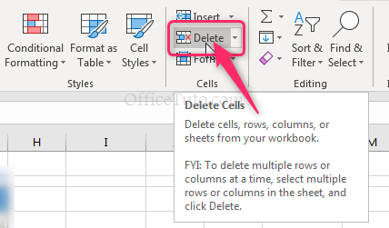
Excel will directly delete the selected cells. Here is the result of this operation from my example:

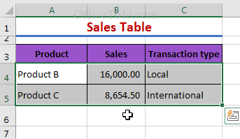
Note: Pay attention when dealing with the deletion of cells as it may cause some disorder in your table if you don’t do it properly. If that occurs, you may need to correct the problem by merging some cells or maybe by discarding the deletion of the cells and, instead of that, delete just their content. Anyway, I think you’ll know then what to do!

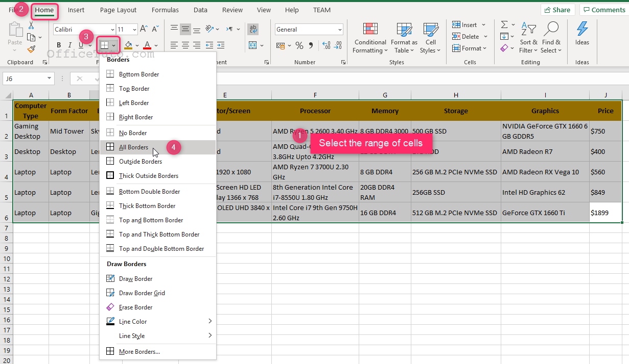
e- How to apply borders to Excel cells

If you’re a beginner and work with an Excel sheet, you may think that the grid that constitues the cells is a real one and can be printed; well, this isn’t the case, and if you need a real table with printable borders, you need to apply these ones to your cells.

Fortunately, this is very easy:

So, to apply borders to a range of cells  start by selecting it, then go to the “Home” tab of the ribbon and, in the group of commands “Font”, click on the “Borders” drop-down list and choose the option you want: “All Borders” would be a good start for you.

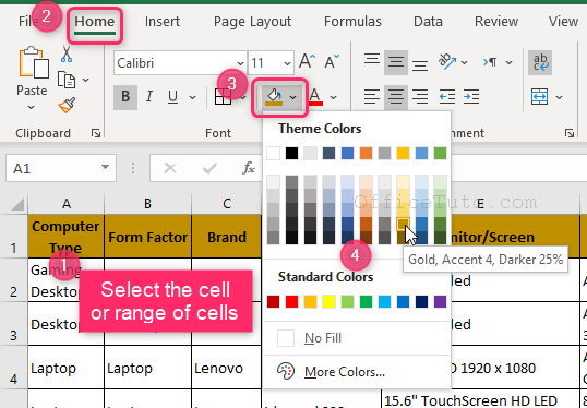
f- How to color cells background

As you may noticed from the previous example in B-5.e “How to apply borders to Excel cells”, the labels (titles) of my table columns have a colored background to better showcase them.

Here is how to do it:

Start by selecting the range of cells you want to fill their background by a color → Go to the “Home” tab of the ribbon and, in the group of commands “Font”, click on the “Fill Color” drop-down list and choose the background color you prefer.

9- How to perform calculations using formulas and functions

One of the most important features provided by Excel is the ability to use formulas and functions to make calculations.

• What are Excel formulas and functions 

The first thing you need to know about Excel formulas and functions is that formulas are a feature more general than functions, since functions can’t be without being used in a formula; meaning I can have a formula without a function, but the opposite is impossible.

Excel functions are built-in codes provided by Excel to perform a specific task, and are used in formulas.

An Excel formula needs to start with the equal (=) sign, and can contain mathematical operators (+, -, *, /, ^) and operands (values, cells references, functions).

When you finish entering your Excel formula, you need to validate it by pressing “Enter” key of the keyboard or clicking the “checkmark” on the left of the “Formula Bar”.

• Types of Excel formulas 

There are 2 types of formulas in Excel: Simple formulas, and formulas with functions.

• Examples of simple Excel formulas:

=(129.58*85)-36.94

=A2+A3+A4

• Examples of Excel formulas with functions:

=SUM(A2:A4)

=PRODUCT(B2:B10)/E2

• Where to enter Excel formulas 

Excel formulas can be entered into the result cell itself; or, after selecting the result cell, in the “Formula Bar”.

• How to create a formula in excel

To create a formula in Excel, you have 2 ways to do:

– Manually: Enter the formula manually in the result cell or in the Formula Bar. This method can be used for simple Excel formulas, as well as for formulas with functions.

– Or, use the “Insert Function” features of Excel. This method is for formulas with functions.
The “Insert Function” feature is accessible from 3 places:

⇒ The “Home” tab of the ribbon in the “Sum” drop-down list:

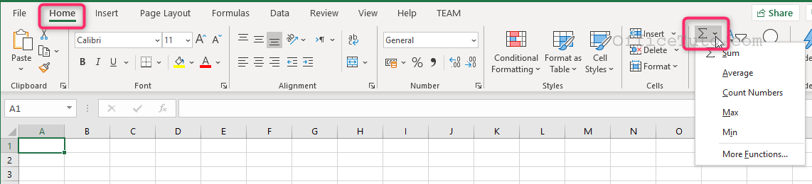
⇒ The “fx” button left to the “Formula Bar”:

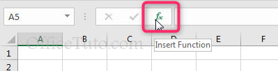
⇒ And in the “Formulas” tab of the ribbon:

• An example of Excel formulas in a dataset

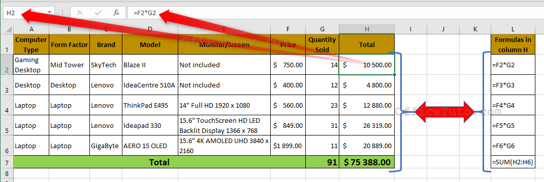
In the following example, I am using formulas to calculate the totals in column H:

– Each cell from column H in the range of H2:H6 is a product of its two equivalents in column F and G.
– And, cell H7 is the sum of cells H2 through H6.
– See the illustration of these formulas in column L. Column L, of course, is not necessary to the dataset and its calculations; it’s just there for the tutorial purposes, so you understand better.

• More on Excel formulas and functions

As you can notice, there are a lot of features regarding this topic of Excel formulas and functions that really go far beyond the scope of this Excel tutorial for beginners; so I won’t go further here but will refer you to a dedicated tutorial that really details all you need to know about Excel formulas and functions: the “Excel formulas and functions” tutorial.

10- How to sort data in Excel

Sorting data in Excel is one of the most useful features that can allow you to sort numbers, dates, and text (full text or mixed with numbers).

To sort your data in Excel, just click on a cell from the range of cells you want to sort → Then:

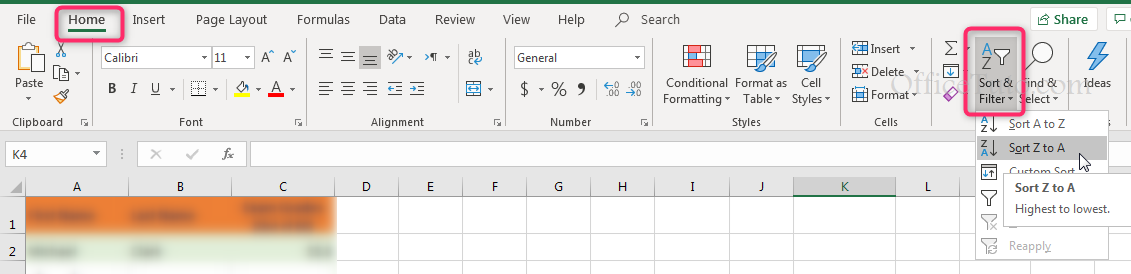
• Go to the “Home” tab of the ribbon and in the group of commands “Editing”, click on the “Sort & Filter” drop-down list and choose the option you need.

Or,

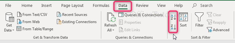
• Go to the “Data” tab of the ribbon, and in the group of commands “Sort & Filter”, choose the option you want.

You’ll notice that the sorting commands change their names according to the format of data to sort. This is because Excel automatically detects the format of data and provides accordingly the right sorting command; meaning:

• If you have text data (or text mixed to numbers), the commands will show in their tooltips the labels “Sort A to Z” and “Sort Z to A“.
• If you have numbers, the commands will show in their tooltips the labels “Sort Smallest to Largest” and “Sort Largest to Smallest“.
• If you have dates, the commands will show in their tooltips the labels “Sort Oldest to Newest” and “Sort Newest to Oldest“.

Let’s take an example of an Excel table containing a list of students names and their grades:

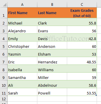
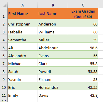
I want to sort my students by their grades, from the highest grade to the lowest one:

So, I click on a cell from the range of cells C2:C11; then, I choose the option “Sort Largest to Smallest” from the “Sort & Filter” command of the “Home” tab.

Excel immediately sorts my list by the Grade column, and here is the result:

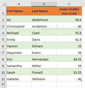
If I want to sort alphabetically my table by students names (last names), I would click on a cell from the range of cells B2:B11; then, I choose the option “Sort A to Z” from the “Sort & Filter” command of the “Home” tab.

Excel would immediately sort my list by the Last Name column, and the result would be as the following:

This was a brief overview of the Excel sorting feature. I showed you here some of its basic tools; you can check out the dedicated tutorial “How to sort data in Excel” where I discuss the sorting commands in much more detail.

11- How to filter data in Excel

This is another amazing feature from Excel; it allows you to filter a part of your data based on a criterion you choose from your columns.

To better illustrate this feature, I will use the following example of an Excel list of computers:

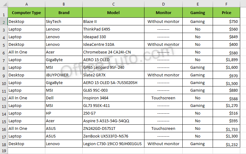
So, let’s say I want to show on my list only “Gaming computers”:

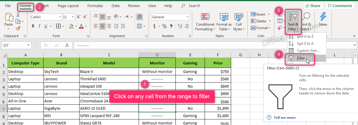
I will start by clicking any cell from my list → Then I will go to the “Home” tab of the ribbon and click in the group of commands “Editing” on the drop-down list “Sort & Filter” and choose “Filter“;

OR,

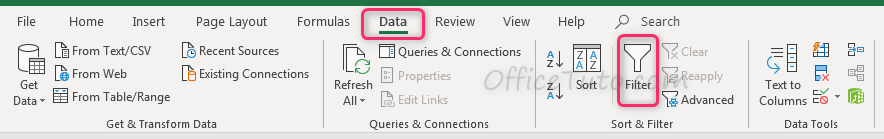
I will go to the “Data” tab and click in the group of commands “Sort & Filter” on the command “Filter“.

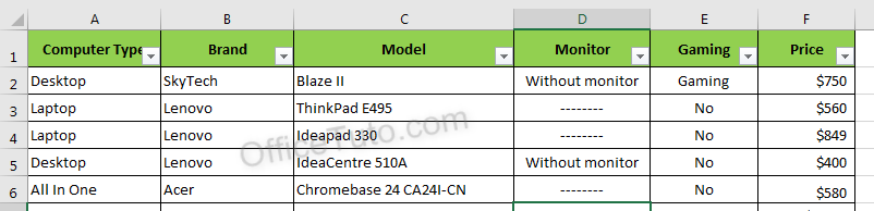
Excel will immediately put vertical arrows as selectors/filters on each header of my columns as illustrated below:

Since I want to show only computers with “Gaming” feature, I will click on the arrow of “Gaming” column (Column E) → Excel displays the drop-down list (illustrated below) where I will uncheck all other options except the one I want, which is option “Gaming”, and click OK.

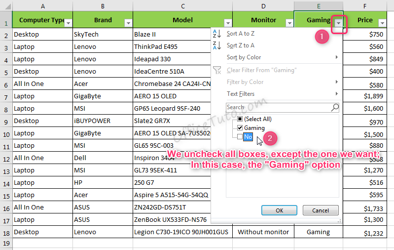
Excel immediately filters my list based on the criterion I have chosen (“Gaming” option) and displays a “Filter icon” on the arrow of the filtered column; see the result below:

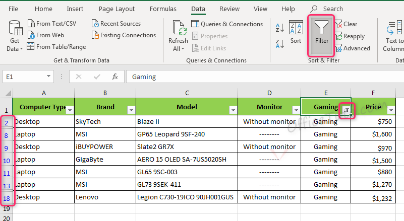
As you can notice from the screenshot above, you can easily verify if a filter is applied and on which column:

See the highlight on the “Filter” command, the arrows on columns labels (see “Gaming” column), and the numbering gaps in the rows headings.

To unfilter or cancel the filter of my column, I just need to click again on the same “Filter” command from “Home” or “Data” tabs.

This was a brief overview of the filter feature in Excel; you’ll find more on the advanced options of the Excel filter in the dedicated tutorial “How to filter data in Excel“.

12- How to create and manage charts in Excel

You can easily create a chart in Excel using the “Insert charts” feature provided in the ribbon.

But, before learning how to create charts in Excel, let’s first introduce the different chart types provided by Excel and which one to choose to better visually and logically represent our data. Then, I will show you how to create a chart, how to move it within a spreadsheet or to another one, and how to change its type, design or format.

a- What are Excel chart types and which one to choose

There are a lot of Excel charts types, but the right type of chart to select depends on the data you have and which aspect you want to highlight. Here are the most common of Excel charts:

• Column charts:

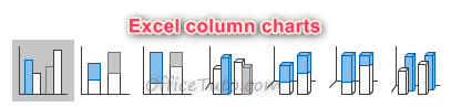
Excel column charts are used to compare data values from a few categories.

• Bar charts:

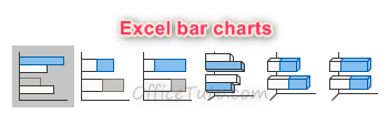
Excel bar charts are used to compare data values from a few categories when you wan to highlight duration or when the text of categories is long.

• Line charts:

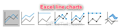
Excel line charts are used to show trends over time or over categories.

• Area charts:

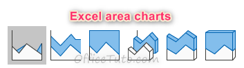
Excel area charts are used to show trends over time or over categories with highlighting the magnitude of change.

• Pie charts:

Excel pie charts are used to show proportions of a whole (proportions from a total of 100%).

• Histogram charts:

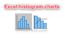
Excel histogram charts are used to show the distribution of the data grouped into bins or ranges. Each column you see in the chart is an illustration of a bin or range of values, rather than of a single value.

• Funnel charts:

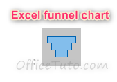
Excel funnel charts are used to show progressively smaller stages in a process; i.e. to show progressively decreasing proportions of values.

• Stock charts:

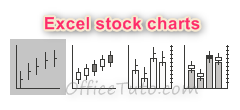
Excel stock charts, as their name suggests, are used to show the trend of a stock’s performance over time.

• Combo charts:

Excel combo charts, as their name suggests, are combination charts used to highlight mixed types of data with different types of charts combined in a same one; e.g. a combo chart with columns and lines, or with columns and area…

b- Create a chart in Excel

Let’s take the following example of a list of computers sales:

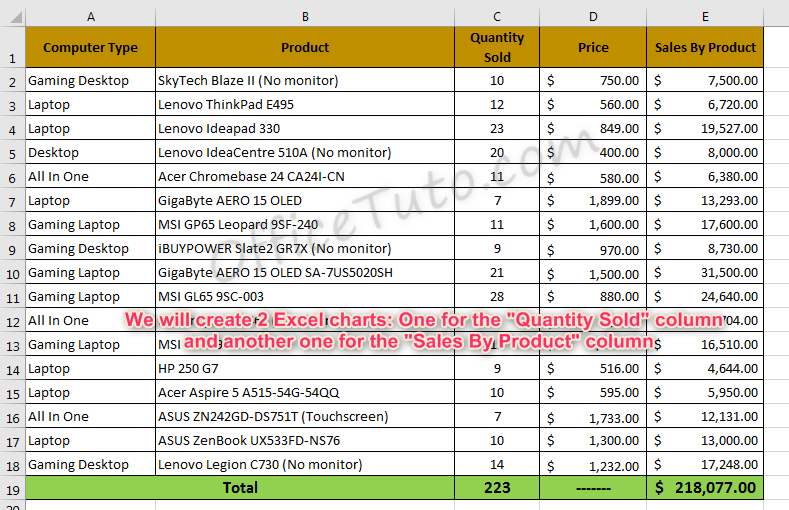
I want to create an Excel chart for the Quantity sold by product, and another one for the Sales by product.

Let’s start with the first Excel chart:

– Create an Excel column chart for the quantity sold by product:

I need to select the range of cells B1:C18 where I have the needed information (Product name and Quantity sold) → Then, go to the “Insert” tab of the ribbon and, in the group of commands “Charts”, select the type of chart I want.

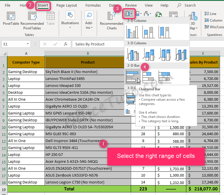
I chose, for this example, a “3-D Clustered Column”.

Excel immediately creates for us the following column chart:

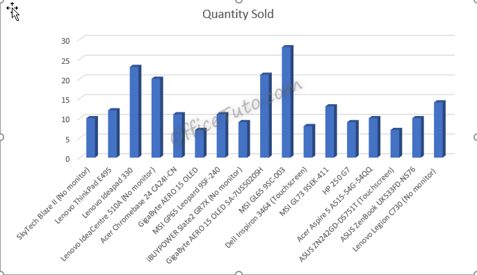
It’s not yet completely set up (we’ll see more later), but it’s a great result for a few clicks of a mouse.

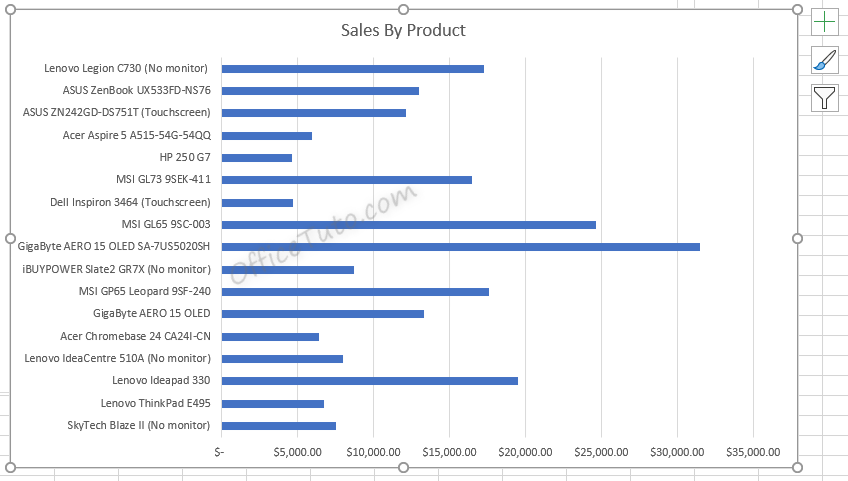
– Create an Excel bar chart for the sales by product:

I will do the same as I did for the “Quantity Sold” chart.

So, I select the range of cells B1:B18 and E1:E18 representing respectively my information from the “Product” and the “Sales by Product” columns. Yes, they are separated ranges of cells, but we learned from section 7-a3 how to select non-adjacent columns; OK, I’ll help you: just select the first range of cells, hold down the “Ctrl” key of the keyboard and select the second range.

Note: I could have selected the whole range of cells B1:E18, but Excel will then include in the charts all the data from the 3 columns “Quantity Sold”, “Price”, and “Sales By Product”, which is not what I need; and then, I would had to modify the data source for the chart in order to represent only the “Sales By Product” column.

Then, I go to the “Insert” tab of the ribbon and, in the group of commands “Charts”, select the type of chart I want.

Here, I will use a different type of chart: even though the “Column chart” would do the work, but I will choose for this second one the “Bar chart” as this type is more convenient for categories with long text, which is my case with the “Product names”.

I chose the “2-D Clustered bar” chart and Excel immediately creates it for me; here is the result:

Here again, there are some settings that can be applied to the chart to make it visually more rich and representative; that’s what we’ll see in the following sections.

c- Move an Excel chart within the same sheet or to another one

• To move an Excel chart within the same sheet:

Just click on the empty area containing it (the chart area) and, when the mouse cursor turns into a double arrow, drag and drop the chart where you want.

• To move an Excel chart to another sheet of the workbook:

Right-click on the chart area (the empty area containing it) and click on “Move Chart“. Excel displays the “Move Chart” dialog box where you can specify where you want your chart to be placed in (a new sheet or an existing one of your workbook).

d- Change the type of a chart in Excel

If you’re not happy with the type of the Excel chart you created and want another type, you don’t need to delete your chart and create a new one:

Just click on your chart → The “Chart Tools” tabs are added to Excel ribbon: In the “Design” tab, go to the “Type” group of commands and click on “Change Chart Type” → Excel displays the “Change Chart Type” dialog box where you can choose a new type for your chart.

e- Change the design and format of a chart in Excel

You can change the design and format of an Excel chart by using the “Design” and “Format” tabs of the ribbon.

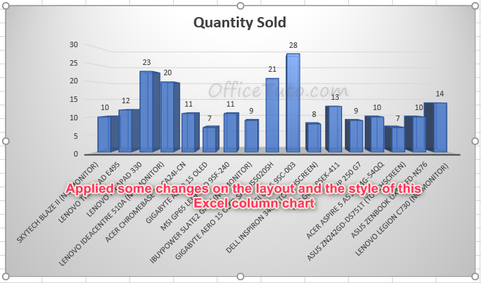
– In the “Design” tab, you can change the layout of the chart (i.e. display or not the title, the legend, the gridlines…), its colors and style.

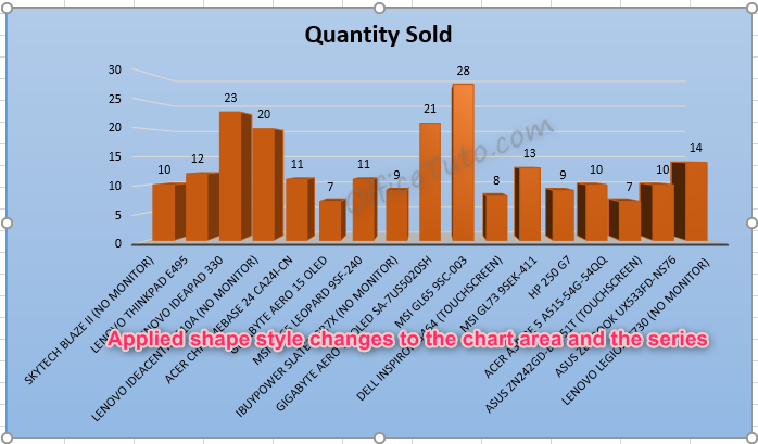
For example, I got the result below for the “Quantity Sold” chart, using the Design tab, by applying the “Layout 2” (to display the data values on the columns) and deleting the legend since I don’t need it, having just one category; I also applied the “Style 3“.

– In the “Format” tab, you can select the element you need and change its fill, outline, or effect.

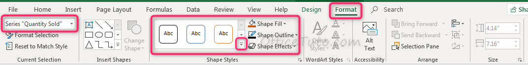
I got the result below for the “Quantity Sold” chart, using the Format tab, by applying a shape fill and shape outline with color “Orange, Accent 2, Darker 25%” to the series, and the shape style “Subtle Effect- Blue, Accent 5” to the chart area.

13- How to print an Excel spreadsheet or part of it

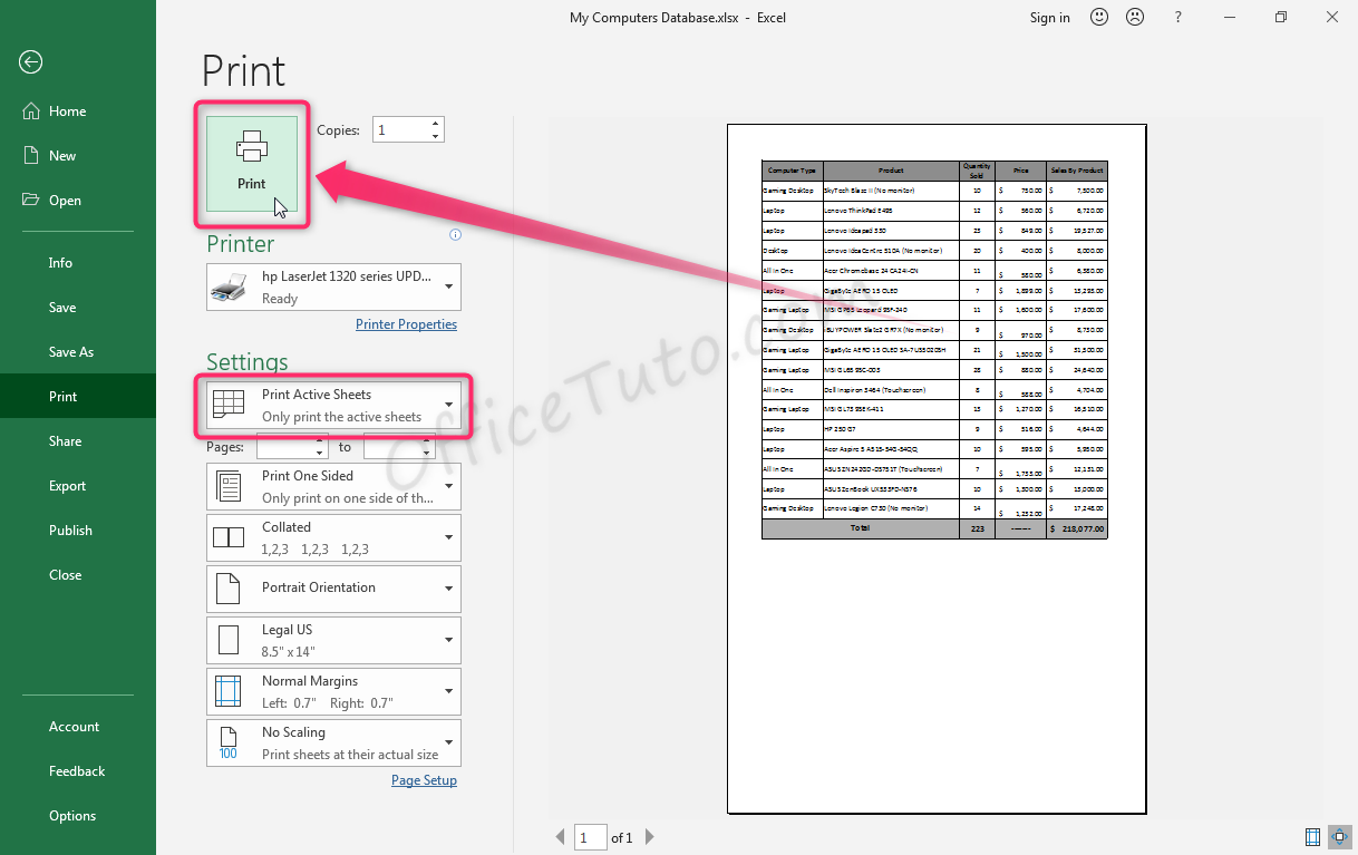
If you want to print just a part of your data, select it; otherwise (printing all data), do nothing and continue with the following:

Go to “File” (or “Office Button” for Excel 2007), then “Print“; or just use the keyboard shortcut “Ctrl + P“.

Excel opens a pane with the printing settings on the left side and a preview of your sheet on the right side.

Note in the top of the settings how you can choose if you want to print the active sheet or just a selection from it.

If everything is OK for you (meaning, the preview shows exactly what you want to print), click on the “Print” button to the top-left.

Conversely, If something is wrong in the preview; for example, the printed area is too big to fit into the paper size (the preview shows only a part from what you want to print), or the printed part appears too small to the whole preview:

Just adjust the width of columns or the height of rows, so the printed part fits exactly to the whole preview.

There are other solutions to this problem, but let’s stick with this solution for this tutorial. We’ll see the advanced methods in another tutorial on this website.

14- How to hide and unfold Excel ribbon

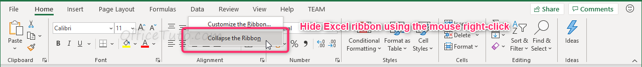
a- How to hide Excel ribbon

Excel ribbon can be hidden to show more of the below area and make more room for your working space.

This can be done by:

• Clicking the “Collapse the ribbon” icon in the bottom right corner of the ribbon;

• Or, by double-clicking on any tab name of the ribbon;
• Or, by right-clicking anywhere on the ribbon and choosing “Collapse the Ribbon“.

♦ The hidden Excel ribbon ♦

The ribbon is then hidden, showing only the tab names, as illustrated below.

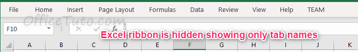
Just keep in mind that you can all the time use a ribbon in its hidden status by clicking on the tab name you want to use; this will momentarily display the tab for you to use its commands. The ribbon will be hidden again once you’re done with it.

b- How to unfold or expand a hidden Excel ribbon

To expand or unfold an already hidden Excel ribbon, you can just double-click on any tab name, or you can right-click anywhere on the ribbon and uncheck “Collapse the Ribbon” command.

15- How to convert an Excel spreadsheet to PDF

To convert an Excel sheet to PDF, go to “File” (or “Office Button” for Excel 2007) and click on “Export“, then on “Create PDF/XPS” → In the “Publish as PDF or XPS” dialog box, enter the name you want for your document and click “Publish“.

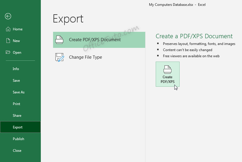
– For Excel 2007:

Excel 2007 (as all other Office 2007 applications) doesn’t have this feature by default; so, if it is your case, you need to add it by downloading and installing this add-in: Microsoft Save As PDF And XPS.

Note: For more details on how to convert an Excel spreadsheet to PDF and all the ways available, check the “4 Ways To Convert Excel to PDF Without Converter Software” tutorial.

16- How to customize the Quick Access Toolbar

The Quick Access Toolbar is the toolbar standing by default on the top of your Excel workspace, in the title bar.

The purpose of this toolbar is to provide quick and easy access for the user to frequently used commands; but the problem is that it comes by default with only 3 buttons: Save, Undo, and Redo.

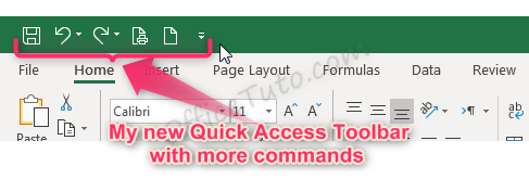
The good news is that you can easily customize it and add or remove whatever command you need. You can also change its location to show it below the ribbon.

• To add commands to the Quick Access Toolbar or remove them from it:

Click on the arrow to its right; the Quick Access Toolbar is expanded.

You’ll notice that the commands currently present in the toolbar are marked with a check-mark, and the non present aren’t marked.

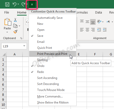
Click on the command you want to add or remove.

Note the “More Commands” option to the bottom of the drop-down list that allows you of course to add more commands than provided here in the list.

I usually add the “Print Preview” and “New” commands to the Quick Access Toolbar because I use them frequently; but it’s up to you to add the commands you think more useful for you; maybe, the “Spelling” or the “Sort” commands, or whatever you need frequently.

• To change the location of the Quick Access Toolbar:

Click on the arrow of the Quick Access Toolbar and choose “Show Below the Ribbon“.

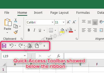
Personally, I don’t really like placing the Quick Access Toolbar at this location as it reduces my workspace, but you might find it useful to have handy commands very close to your workspace, instead to go search them in the ribbon.

Conclusion

This was the Excel tutorial for beginners; I tried to include in it all the basics and common features of Excel that would help you in your first steps to master Excel.

I hope you’ll find it very useful.

Of course, to get the most out of this tutorial, don’t just read it, but apply all the information in it, step by step. If you can’t do it all at once, bookmark this page in your browser and practice at your own pace.

- "Learn Excel: For Beginners" Series Navigation:

2: Cell Format Types in Excel and How To Implement Them >>