How to Sort Data in Excel

Sorting data in Excel is one of the most useful features provided by this software.

Excel offers options to sort data either numerically, alphabetically, by date, or by other options depending on the field type being sorted.

There are two types of Excel sort: the simple sort and the custom sort. The simple sort allows to only sort a column by cell value, while the custom sort allows to sort a column, multiple columns, a row, multiple rows, sort by cell color, by font color, by conditional formatting icon, and perform a case sensitive sort.

A- Sort a column in Excel using the Simple sort

The simple Excel sort commands are provided into two tabs of the ribbon: the “Home” tab and the “Data” tab.

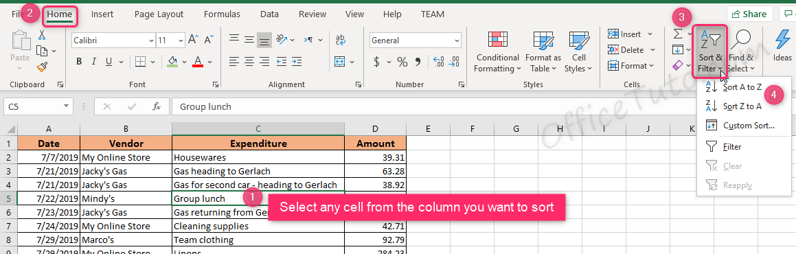
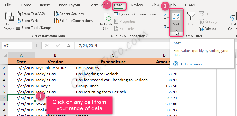
So, to sort a column in Excel:

• Click on any cell within that column.
• Go to the “Home” tab of the ribbon.
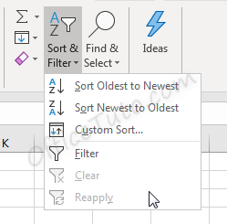
• In “Editing” group, click on “Sort & Filter”.
• Choose one of the two first commands.

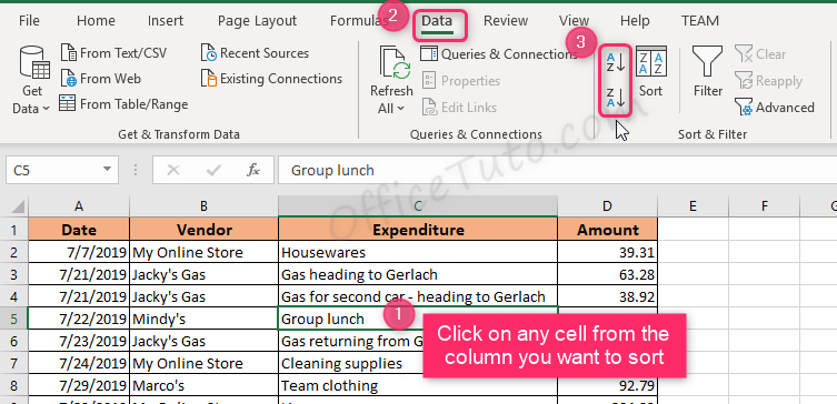
Or, you can also:

• Click on any cell within that column.
• Navigate to the “Data” tab of the ribbon.
• Go to the “Sort & Filter” group of commands.
• Click on one of the two sort commands.

Excel will then immediately adjust the data following the order you specified; and of course, it keeps consistent your data by moving the entire rows and not just the cells of the selected column.

Note about the labels of the Excel sort commands:

The labels of Excel sort commands differ depending on the data type of the column by which we are sorting our data: text, numbers, or dates.

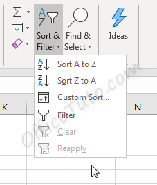
• If it is a column of text (or text mixed to numbers), Excel sort commands are labeled “Sort A to Z” and “Sort Z to A”.

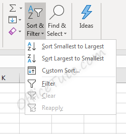
• If it is a column of numbers, Excel sort commands are labeled “Sort Smallest to Largest” and “Sort Largest to Smallest”.

• If it is a column of dates, Excel sort commands are labeled “Sort Oldest to Newest” and “Sort Newest to Oldest”.

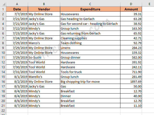
Let’s now apply all of this on an example containing the three types of data, text, numbers, and dates:

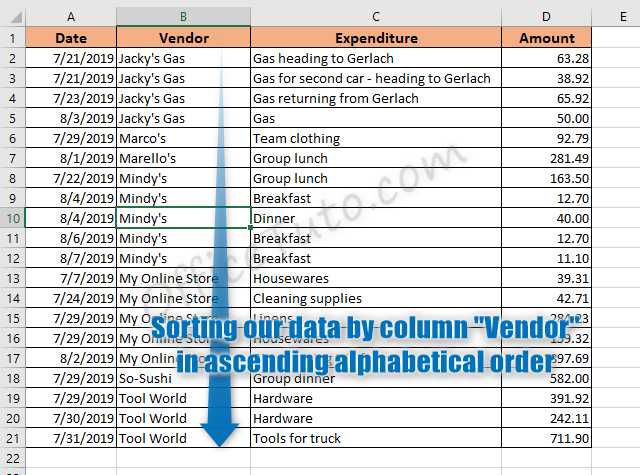
• To sort our data by Vendor, in ascending alphabetical order:

We click on a cell from the column “Vendor” and click on the “Sort A to Z” command from “Home” tab or “Data” tab of the ribbon.

The result is illustrated in the following screenshot:

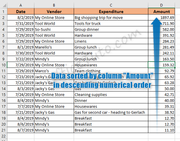
• To sort our data by Amount, in descending numerical order:

We click on a cell from the column “Amount” and click on the “Sort Largest to Smallest” command from “Home” tab or “Data” tab of the ribbon.

The result is illustrated in the following screenshot:

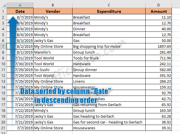
• To sort our data by Date, in descending order:

We click on a cell from the column “Date” and click on the “Sort Newest to Oldest” command from “Home” tab or “Data” tab of the ribbon.

The result is illustrated in the following screenshot:

Important note about the consistency of data after Excel sort:

Because there are adjacent cells with related information pertinent to the rows being sorted, these rows are sorted by default as well. So, be careful when using a simple sort, as Excel may not perform this action by default.
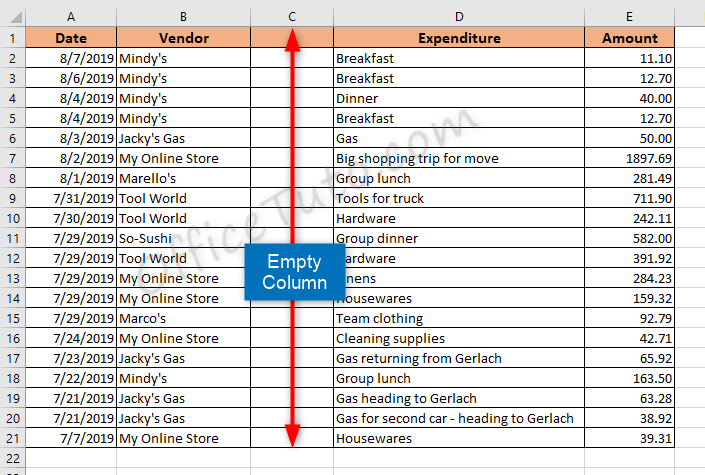
For example, if there was an empty column with no title separating Vendor and Expenditure, Excel would have assumed the information to the right of vendor (separated by a null column) to be a separate data set, and the information would not have been sorted.

Example before sorting by Vendor where there is a null column to the right of the Vendor column:

Example after sorting by Vendor (A to Z) where there is a null column to the right of the Vendor column:

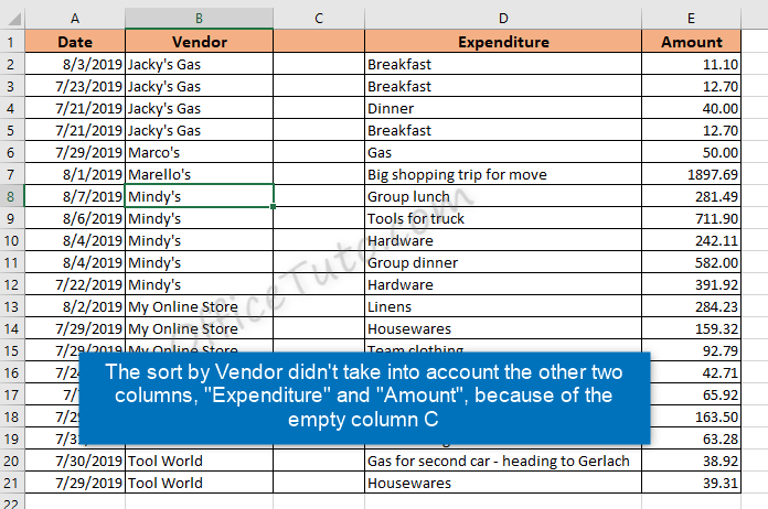
Notice that the information in the columns for Expenditure and Amount were not adjusted, because of the existence of the empty column.

B- Sort Excel columns or rows using Custom Sort

The Custom sort feature in Excel is a more advanced feature than the simple Excel sort and allows more flexibility. The custom sort of Excel allows to sort a column, multiple columns, a row, multiple rows, sort by cell color, by font color, by conditional formatting icon, and perform a case sensitive sort.

The Excel custom sort command is available in two tabs of the ribbon: the “Home” tab and the “Data” tab.

So, to perform a custom sort in Excel:

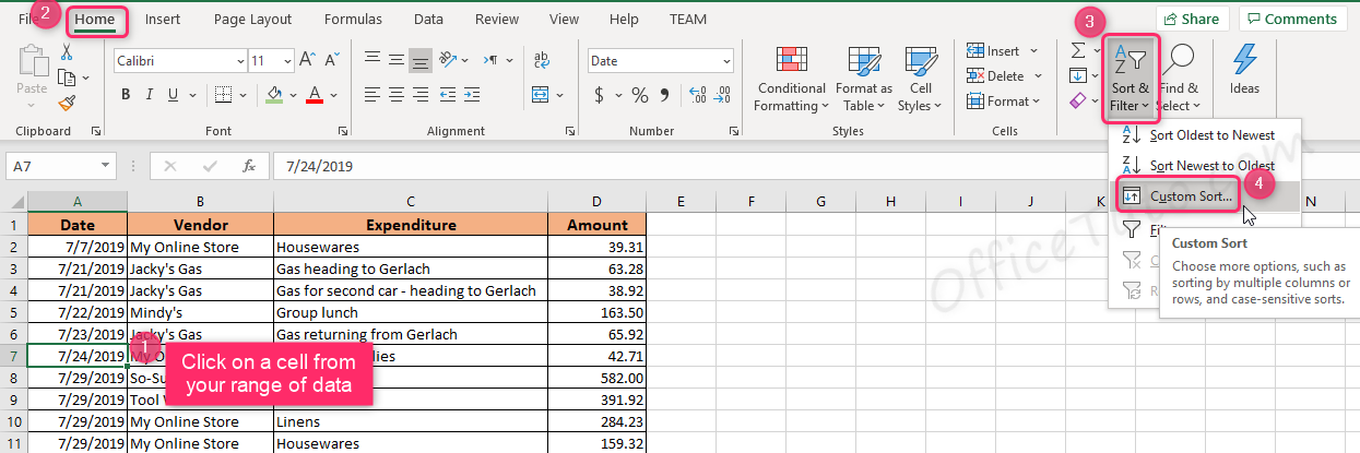
1. Click on a cell in the range you want to sort.
2. Then go into the “Home” tab.
3. Go to the group of commands “Editing”.
4. Click on the “Sort & Filter” drop-down list.
5. Click on the “Custom Sort” command.
6. The Sort dialog box will display.
7. Set the options from the drop-down lists.
8. Click on “OK” to sort your data.

Or, you can also:

1. Click on a cell in the range you want to sort.
2. Go into the “Data” tab.
3. Go to the group of commands “Sort & Filter”.
4. Click on “Sort” command.
5. The Sort dialog box will display.
6. Set the options from the drop-down lists.
7. Click on “OK” to sort your data.

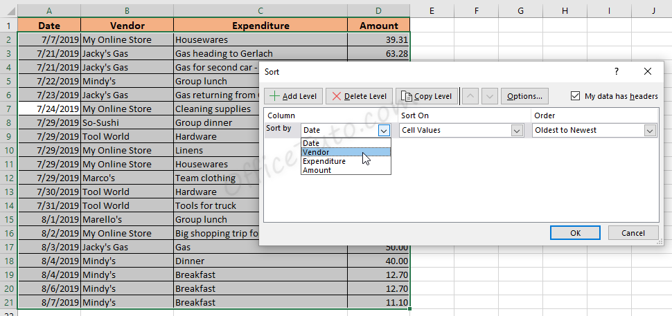
The “Sort” dialog box provides the following options:

– The three drop-down lists: which column or row to sort by, the criteria to sort on, and the sort order.
– The levels buttons (Add level, Delete Level, Copy Level, Move Up Level, and Move Down Level).
– The check-box “My data has headers”.
– And the “Options” buttons.

Let’s detail each option of the “Sort” dialog box in the following:

• “My data has headers” check box: If it’s not already checked, it’s always recommended to start by checking “My data has headers” check box, so you get your labels (or titles) of columns displayed in the “Sort by” drop-down list, which will make easier your work in the “Sort” dialog box.

• “Sort by” drop-down list (which column or row to sort by):

This drop-down list displays all adjacent columns or rows with headers from your range of cells. Click on the name of the column or the row you want to sort your data by.

Note: Sorting by rows is available in the “Options” button on this dialog box, where you would need to check the “Sort left to right” option (see the dedicated section later in this tutorial).
Of course, your data should be logically organized by rows for this option to work as expected.

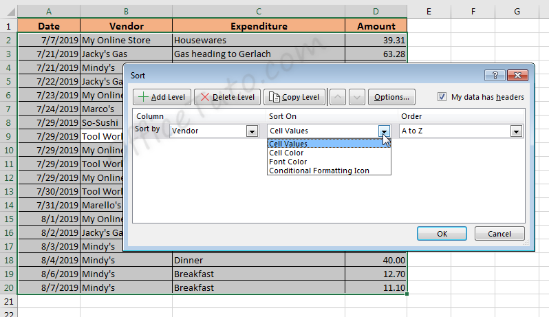
• “Sort On” drop-down list (provides the criteria to sort on):
  • Cell Values: This will function in the same way as the simple sort and sort either alphabetically, by date, or from smallest to largest number.
  • Cell Color: Sorts by fill color of the cells in the column being sorted.
  • Font Color: Sorts by color of the font of the cells in the column being sorted.
  • Conditional Formatting Icon: Sorts by conditional formatting applied to the cells.

• “Order” drop-down list: Choose here the order of the Excel sort you want. The order options provided here will depend on the option selected in the “Sort on” drop-down list.
  So, it will be:
  – “A to Z” and “Z to A”: if the “Sort On” drop-down list is set on “Cell values” and your column or row values are text.
  – “Smallest to Largest” and “Largest to Smallest”: if the “Sort On” drop-down list is set on “Cell values” and your column or row values are numbers.
  – “Oldest to Newest” and ‘Newest to Oldest”: if the “Sort On” drop-down list is set on “Cell values” and your column or row values are dates.
  – A color: if the “Sort On” drop-down list is set on “Cell Color” or “Font Color”; assuming of course that a color was already applied to the cells or the font.
  – An Icon: if the “Sort On” drop-down list is set on “Conditional Formatting Icon”; assuming of course that a conditional formatting by icon was already applied.

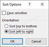
• “Options” button: When clicking on this button, Excel provides you with two additional sort options: the case sensitive sort and the sorting by rows (sort left to right).

• “Add Level”, “Delete Level”, and “Copy Level”: You will need these options when sorting multiple columns or rows (see the following sections). You will add a level (another level of sorting) to sort by an additional column (or row); you will delete a level when you no longer need to sort by a particular column (or row); and, you’ll copy a level to speed up your work when adding a level similar to a previous one.

Now that we know how to use the custom sort in Excel, let’s apply that in the examples of the following sections:

1- Sort multiple columns in Excel using the custom sort

To sort multiple columns in Excel, you need of course to have equal values in one or many subsequent column(s), so you can have multiple columns sorted at the same time.

Let’s take the following example and try to sort our data, first by “Vendor” in ascending order, then by “Amount” in descending order for same vendors:

So, to sort by multiple columns in Excel:

1. Click on any cell from your range of data.
2. Click “Sort” in “Sort & Filter” of “Data” tab.
3. Excel displays the “Sort” dialog box.
4. Select the column you want in the “Sort by”.
5. Set the “Sort On” and “Order” options.
6. Click on the “Add level” button at the top.
7. Set the second column, Sort On, and Order.
8. And so on. When finished, click on “OK”.

In my example, as illustrated below, I first sort by “Vendor”, on “Cell Values”, with an ascending alphabetical order (A to Z). Then, I click on the “Add level” button to add the second level of sorting, and I sort by “Amount”, on “Cell Values”, in descending numerical order (Largest to Smallest).

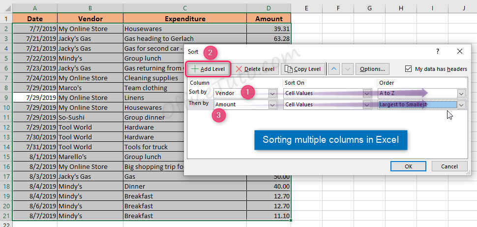
Note that my range of data has header columns, so I keep checked “My data has headers” checkbox. If the range of data being sorted does not have a header column, I’ll need to uncheck the box “My data has headers” to display the column letter in the “Sort by” field instead of displaying the value (header) from the first row of the data set.

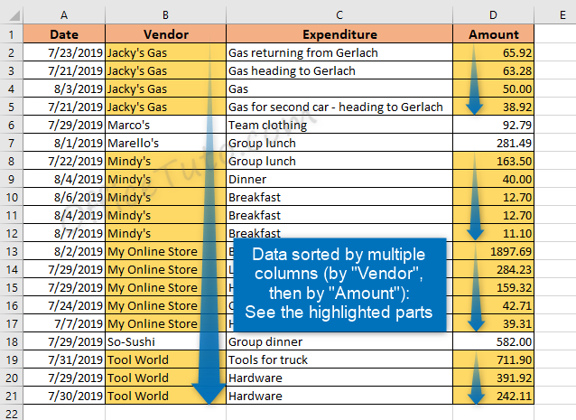
When I click on “OK”, Excel sorts my data first by “Vendor”, then for same vendors, sorts by “Amount”, as illustrated in the screenshot below (I highlighted the relevant parts for more comprehension).

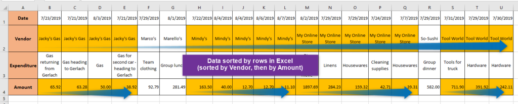
2- Sort data by rows in Excel using the custom sort

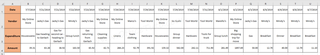
Let’s suppose I have my data organised by rows; meaning, the headers of my range of cells are the labels of the rows (and not the columns); see the following screenshot. And, I want to sort my data; so, I’ll need to do it by rows (and not columns of course) using Excel custom sort.

To sort data in Excel by rows:

1. Select the range without including the headers
2. Click “Sort” in “Data” tab, then “Options”.
3. Check “Sort left to right” and click “OK”.
4. Select the row you want in the “Sort by”.
5. Set the “Sort On” and “Order” options.
6. To sort by more rows, click on “Add level”.
7. Set the second row, Sort On, and Order.
8. And so on. When finished, click on “OK”.

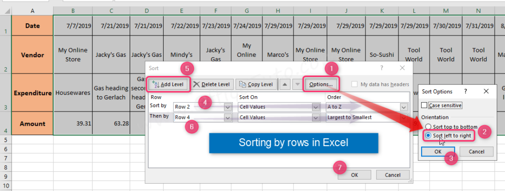
In my example, as illustrated below, I select my range of cells without including the headers “Date”, “Vendor”, “Expenditure”, or “Amount”. Then, I use the custom sort with “Sort left to right” option checked to sort by the “Vendor” row (row 2), on “Cell Values”, with an ascending alphabetical order (A to Z). After that, I click on the “Add level” button to add the second level of sorting by rows, and I sort by the “Amount” row (row 4), on “Cell Values”, in descending numerical order (Largest to Smallest).

When I click on “OK”, Excel sorts my rows first by “Vendor”, then for same vendors, sorts by “Amount”, as illustrated in the screenshot below (I highlighted the relevant parts for more comprehension).

Note that in the “Sort by” option of the “Sort” dialog box, Excel doesn’t provide the labels of the rows because it only recognizes the organization in columns; hence, it names them “row 1”, “row 2”, etc.

3- Excel sort by color using the custom sort

For this example, some of the Expenditure cells have been coded, to indicate their importance, either in green (less important), yellow (medium importance), or red (very important).

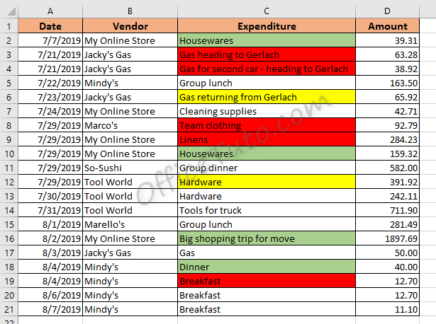
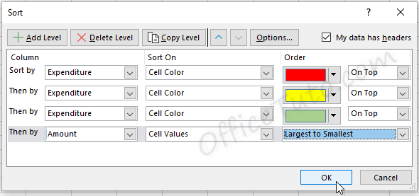
Let’s say I want to see the most important (red) Expenditures listed at the top, then the least important (yellow, then green), and within this want to have the higher Amount items listed higher on the list.

For this, I’ll use a Custom Sort that will allow me to sort by color and to sort multiple columns.

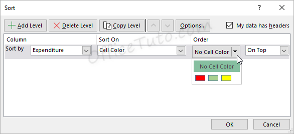
To sort by cell color in Excel:

1. Click on a cell in your data, then on “Sort” in “Sort & Filter” of “Data” tab
2. Excel displays the “Sort” dialog box.
3. Select the column with color in the “Sort by”.
4. Set the “Sort On” on “Cell Color”, and select another color and order in “Order”
5. Click on the “Add level” button at the top.
6. Select the same column with color in “Sort by”
7. Set the “Sort On” on “Cell Color”, and select another color and order in “Order”
8. And so on. When finished, click on “OK”.

To sort by font color in Excel:

1. Click on a cell in your data, then on “Sort” in “Sort & Filter” of “Data” tab
2. Excel displays the “Sort” dialog box.
3. Select the column with color in the “Sort by”.
4. Set the “Sort On” on “Font Color”, and select another color and order in “Order”
5. Click on the “Add level” button at the top.
6. Select the same column with color in “Sort by”
7. Set the “Sort On” on “Font Color”, and select another color and order in “Order”
8. And so on. When finished, click on “OK”.

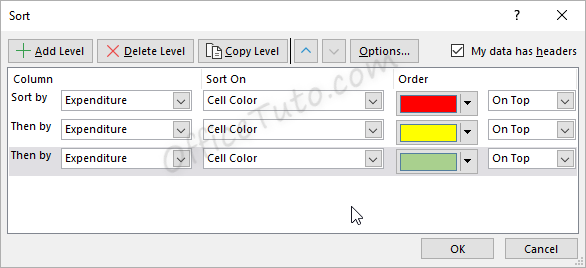
So, applying the above instructions from “Sort by cell color in Excel” on my example: I click on any cell from my range of data, then navigate to Custom sort (in the “Home” tab or the “Data” tab of the ribbon) and add multiple levels in the “Sort” dialog box using the Add Level button.

Note that my range of data has header columns, so I keep checked “My data has headers” checkbox. If the range of data being sorted does not have a header column, I’ll need to uncheck the box “My data has headers” to display the column letter in the “Sort by” field instead of displaying the value (header) from the first row of the data set.

From here, I can click the “Add Level” button to create a new row within the dialog box and updating it with the next set of information. Although, the process can be made easier when creating multiple levels with similar options, by using the “Copy Level” button: Click on an existing level to highlight it. This will then copy the highlighted level (in this case the ones with cell color = red) and recreate it.

I can then simply change the color instead of having to re-update all the fields.

Note that you can use the up and down buttons  to adjust the order of the entries. In my case, no need to use them as I entered the exact order I want.

For this example, I also wanted to sort by Amount, so I can add one additional level for this at the bottom of the list since more importantly I want to sort by color.

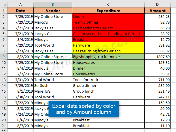
The result of my Excel sort by color and by multiple columns is illustrated below:

4- Case sensitive sort in Excel using custom sort

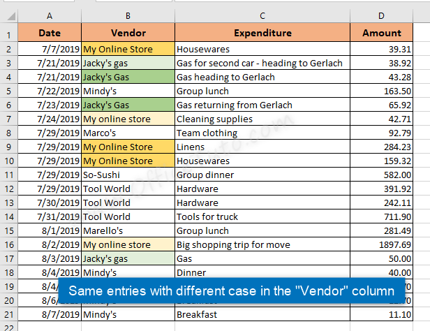
You may need to use the case sensitive sort in Excel if you want to sort columns or rows that contain identical entries with different case (entries that are supposed to be different).

In the range of cells illustrated below, I have two examples of this kind: “My Online Store” vs “My online store”, and “Jacky’s Gas” vs “Jacky’s gas”.

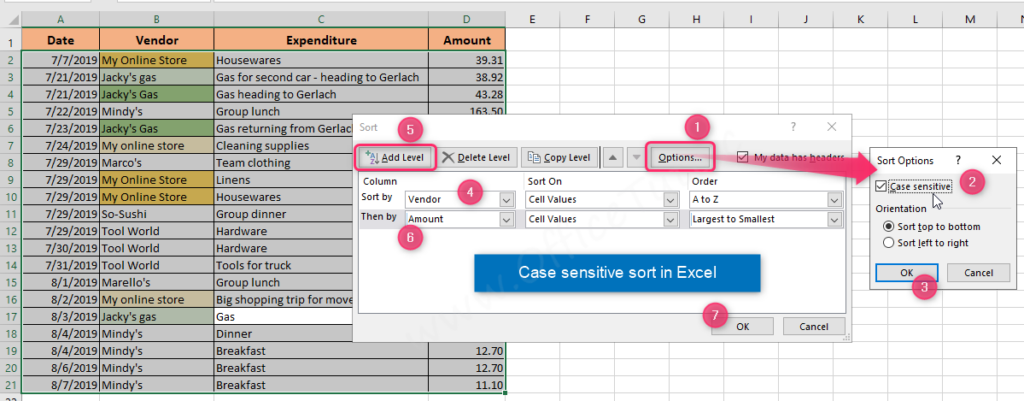
To perform a case sensitive sort in Excel:

1. Click on any cell from your range of data.
2. Click “Sort” in “Data” tab, then “Options”.
3. Check “Case sensitive” option and click “OK”.
4. Select the row you want in the “Sort by”.
5. Set the “Sort On” and “Order” options.
6. To sort by more rows, click on “Add level”.
7. Set the second row, Sort On, and Order.
8. And so on. When finished, click on “OK”.

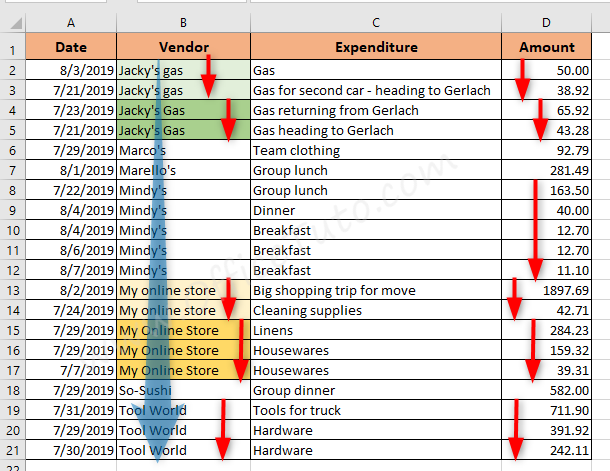
In my example, as illustrated below, I click on a cell from my range of data. Then, I use the custom sort with “Case sensitive” option checked to sort with taking into account the case difference of the identical entries. I start by sorting with the “Vendor” column, on “Cell Values”, with an ascending alphabetical order (A to Z). Then, I click on the “Add level” button to add the second level of sorting, and I sort by “Amount”, on “Cell Values”, in descending numerical order (Largest to Smallest).

Note that my range of data has header columns, so I keep checked “My data has headers” checkbox. If the range of data being sorted does not have a header column, I’ll need to uncheck the box “My data has headers” to display the column letter in the “Sort by” field instead of displaying the value (header) from the first row of the data set.

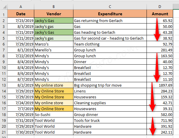
When I click on “OK”, Excel sorts my data first by “Vendor”, then for same vendors, sorts by “Amount”; but it sorts the Vendor column in a case-sensitive way, as you can see in the screenshot below (I highlighted the relevant parts for more comprehension). It placed “Jacky’s gas” instances before “Jacky’s Gas” ones, and “My online store” instances before “My Online Store” ones.

A non case-sensitive sort would give me a different result. So, if I do a normal sorting and don’t check the “cas sensitive” option, the identical entries in the “Vendor” column would be sorted with respect of the descending numerical order of the “Amount” column. See the screenshot below for more comprehension.

C- Wrap up

So, that was the tutorial about Excel sort feature. We saw that there are two types of sort in Excel: the simple sort and the custom sort.

The simple sort is very easy to apply and will be sufficient in the most common tasks where you sort a column by its cells values, whereas the custom sort is for more advanced purposes; so, use either one appropriately, depending on your situation.

- "Learn Excel: For Beginners" Series Navigation:

<< 6: The 4 Ways To Add Numbers in Excel Using SUM Function8: How to Freeze Rows and Columns in Excel >>