The 4 Ways To Join the Content of Cells in Excel

There are four ways to join the content of the cells in Excel: the ampersand operator &, and the functions CONCATENATE, CONCAT, and TEXTJOIN.

The & operator and the CONCATENATE function can be used whatever the Excel version is, whereas The CONCAT and the TEXTJOIN functions are available only in Excel 2019 or newer, and in Excel for Microsoft 365.

In this tutorial, I show you how to join the content of cells in Excel, with and without a separator, using the ampersand operator &, and the Excel functions CONCATENATE, CONCAT, and TEXTJOIN; and at the end, I provide you with a table where I compare the advantages and disadvantages of the four methods, based on different criteria, with an example for each.

A/ Join the content of cells in Excel without a separator

In Excel, there are 4 ways to join the content of two or more cells without a separator: using the ampersand operator &, or one of the functions CONCATENATE, CONCAT, or TEXTJOIN.

The use of ampersand operator & is the fastest and easiest one of these 4 methods when the cells are not adjacent and no separator is needed, while the CONCAT function is the most appropriate when the cells are adjacent and no separator is needed.

1- Join content of cells in Excel without separator using &

To join the content of multiple cells in Excel without a separator (spacing, comma, dash…) using the ampersand operator &:

• Type equal symbol = on the result cell
• Click on the first cell and type ampersand &
• Click on the second cell
• To join content of the 2 cells, press Enter.
• Otherwise, to join content of more cells:
• Type & and click on the other cell
• And so on for all the remaining cells
• Finally, press Enter.

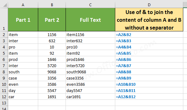
To illustrate how to join the content of two cells in Excel using the ampersand operator &, without adding a separator between them, let’s take the following example where I want to join the content of cells in columns A and B, and put it in column C.

The general syntax is: =first_cell&second_cell

The formula, for example from cell C2, is as follows: =A2&B2

2- Join cells content without a separator using CONCATENATE

The CONCATENATE function is available in all Excel versions, and its syntax is: =CONCATENATE(content1, content2,…).

To join the content of multiple cells in Excel without a separator (spacing, comma, dash…) using the CONCATENATE function:

• Click on the result cell.
• Type the following: =CONCATENATE(
• Click on the first cell and type a comma
• Click on the second cell
• To join content of the 2 cells, press Enter.
• Otherwise, to join content of more cells:
• Type another comma and click on the next cell
• And so on for the remaining cells. Press Enter.

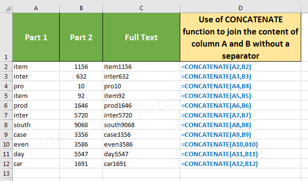
To illustrate how to join the content of two cells in Excel using the CONCATENATE function, without adding a separator between them, let’s take the following example where I want to join the content of cells in columns A and B, and put it in column C.

The general syntax is: =CONCATENATE(first_cell,second_cell)

The formula, for example from cell C2, is as follows: =CONCATENATE(A2,B2)

3- Join cells content without a separator using CONCAT

The CONCAT function is available only in Excel 2019 and newer, or Excel 365. Its syntax is: =CONCAT(content1, content2,…) or =CONCAT(first_cell:last_cell) depending on whether the cells are adjacent or not.

The formula =CONCAT(first_cell, second_cell,…) is for selecting individual cells (especially when not adjacent), whereas =CONCAT(first_cell:last_cell) is for when selecting a range of cells (requires adjacent cells).

– Join Excel cells without a separator, using CONCAT function (adjacent or non-adjacent cells)

To join the content of multiple Excel cells without a separator (spacing, comma, dash…), using CONCAT function for adjacent or non-adjacent cells:

• Type in the result cell: =CONCAT(
• Click on the first cell and type a comma
• Click on the second cell
• To join content of the 2 cells, press Enter.
• Otherwise, to join content of more cells:
• Type another comma and click on the next cell
• And so on for all the remaining cells
• Finally, press Enter.

– Join adjacent Excel cells without a separator, using CONCAT function

To join the content of adjacent Excel cells without a separator (spacing, comma, dash…), using CONCAT function:

• Click on the result cell.
• Type the following: =CONCAT(
• Select the range of cells you want to join
• Press Enter.
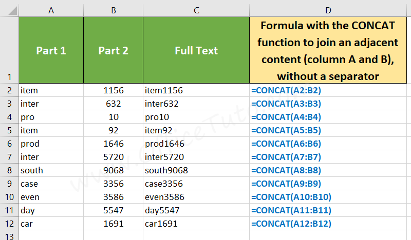
• Resulting formula will be =CONCAT(first_cell:last_cell)

To illustrate how to join the content of adjacent cells in Excel using the CONCAT function, without adding a separator between them, let’s take the following example where I want to join an adjacent content of cells (columns A and B), and put it in column C.

4- Join cells content without a separator using TEXTJOIN

The TEXTJOIN function is available only in Excel 2019 and newer, or Excel 365. Its syntax is: =TEXTJOIN(“delimiter”, ignore_empty_cells, content1, content2,…) or =TEXTJOIN(“delimiter”, ignore_empty_cells, first_cell:last_cell)

The formula =TEXTJOIN(“delimiter”, ignore_empty_cells, first_cell, second_cell,…) is for selecting individual cells (especially when not adjacent), whereas =TEXTJOIN(“delimiter”, ignore_empty_cells, first_cell:last_cell) is for selecting a range of cells (requires adjacent cells).

• The delimiter is the separator to use to separate the content of the joined cells, but since I’m talking here about joining content of cells without a separator, I will just type opening and closing double quotes to indicate non separator, like this “”.
• The ignore_empty_cells is a boolean argument; so, it can be True (to not take into consideration the empty cells) or False (to join the empty cells). Can be useful when you have empty cells at the end of the range, otherwise choose either one.

– Join Excel cells without a separator, using TEXTJOIN function (adjacent or non-adjacent cells)

To join the content of Excel cells without a separator (spacing, comma, dash…) using TEXTJOIN, for adjacent or non-adjacent cells:

• Type in the result cell: =TEXTJOIN(“”,
• Type True or False (ignore or not empty cells)
• Type a second comma and click the first cell
• Type a third comma and click on the second cell
• To join content of the 2 cells, press Enter.
• Otherwise, to join content of more cells:
• Type another comma and click on the next cell
• And so on for the remaining cells. Press Enter.

– Join adjacent Excel cells without a separator, using TEXTJOIN function

To join the content of adjacent cells without a separator (spacing, comma, dash…) using TEXTJOIN:

• Click on the result cell.
• Type the following: =TEXTJOIN(
• Type two double quotes “” (for no separator)
• Type a comma to separate function arguments
• Type True or False (ignore or not empty cells)
• Type a second comma
• Select the range of cells you want to join
• Press Enter.

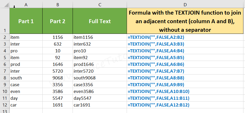
To illustrate how to join the content of two cells in Excel using the TEXTJOIN function, without adding a separator between them, let’s take the following example where I want to join the content of cells in columns A and B, and put it in column C.

B/ Join the content of cells with delimiter (comma, space..)

In Excel, there are 4 ways to join the content of two or more cells with a separator between them: using the ampersand operator &, or one of the functions CONCATENATE, CONCAT, or TEXTJOIN.

The TEXTJOIN function is the most appropriate when one separator is needed, whether the cells are adjacent or not, while the use of ampersand operator & is the fastest and easiest one of these 4 methods when different separators are used.

1- Join content of cells in Excel with a separator using &

The simplest way to join the content of multiple cells in Excel with a separator between them (spacing, comma, semicolon, dash, colon, or any other text) is to use the ampersand operator &.

So, to join the content of multiple cells in Excel with a separator between them, using the ampersand operator &:

• Type equal symbol = on the result cell
• Click on the first cell and type ampersand &
• Type the separator into double quotes
• Type & then Click on the second cell
• Press Enter to join the 2 cells. To join more:
• Type &. Then a separator if any, in double quotes
• Click the other cell. And so on for the rest ones
• Finally, press Enter.

– Join first and last name in Excel using & operator

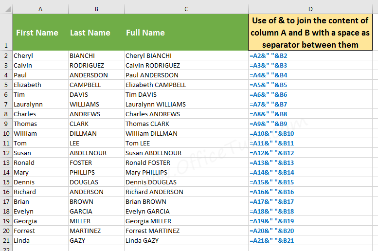
To illustrate how to join the content of two cells in Excel using the ampersand operator &, with adding a separator between them, let’s take the following example where I want to join first and last names from columns A and B, with a space as a separator, and put the result in column C.

In the formula, the space used as a separator is put into double quotes; the syntax of the formula is: =first_cell&”space”&second_cell

The formula, for example from cell C2, is as follows: =A2&” “&B2

– Join 3 Excel cells using & with space and comma separators

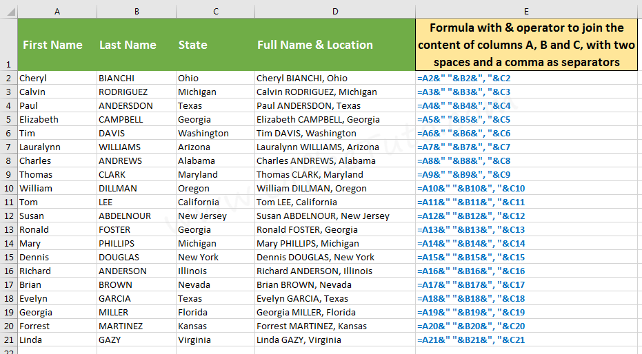
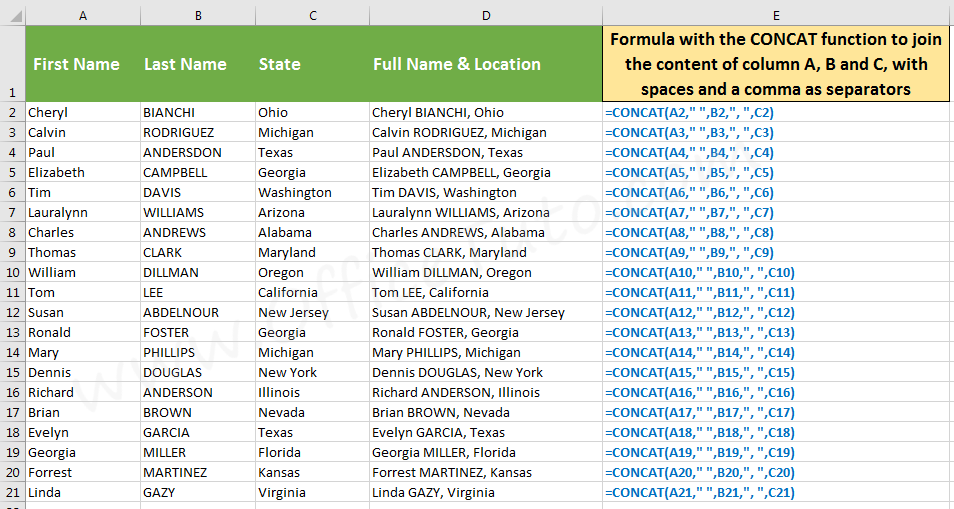
Here is another example where I use the ampersand operator & to join first and last names, and their location (the state) from columns A, B, and C, and a space and a comma as separators; the result is in column E.

In the formula, the two spaces and the comma used as separators are put into double quotes; the syntax of the formula is: =first_cell&”space”&second_cell&”comma space”&third_cell

The formula, for example from cell D2, is as follows: =A2&” “&B2&”, “&C2

2- Join content of cells with a separator using CONCATENATE

The CONCATENATE function is available in all Excel versions, and its syntax when inserting a separator is: =CONCATENATE(content1, “separator”, content2,…)

To join the content of multiple cells in Excel with a separator between them (spacing, comma, semicolon, dash, colon, or any other text), using the CONCATENATE function:

• In the result cell, type: =CONCATENATE(
• Click the first cell and type a comma
• Type the separator into double quotes
• Click the second cell
• To join the 2 cells, press Enter. To join more:
• Type a comma. Then a separator in double quotes
• Click the next cell. And so on for the rest ones
• Finally, press Enter.

– Join first and last name with Excel CONCATENATE function

To illustrate how to join the content of two cells in Excel using the CONCATENATE function, with adding a separator between them, let’s take the following example where I want to join first and last names from columns A and B, with a space as a separator, and put the result in column C.

In the formula, the space used as a separator is put into double quotes; the syntax of the formula is: =CONCATENATE(first_cell,”space”,second_cell)

The formula, for example from cell C2, is as follows: =CONCATENATE(A2,” “,B2)

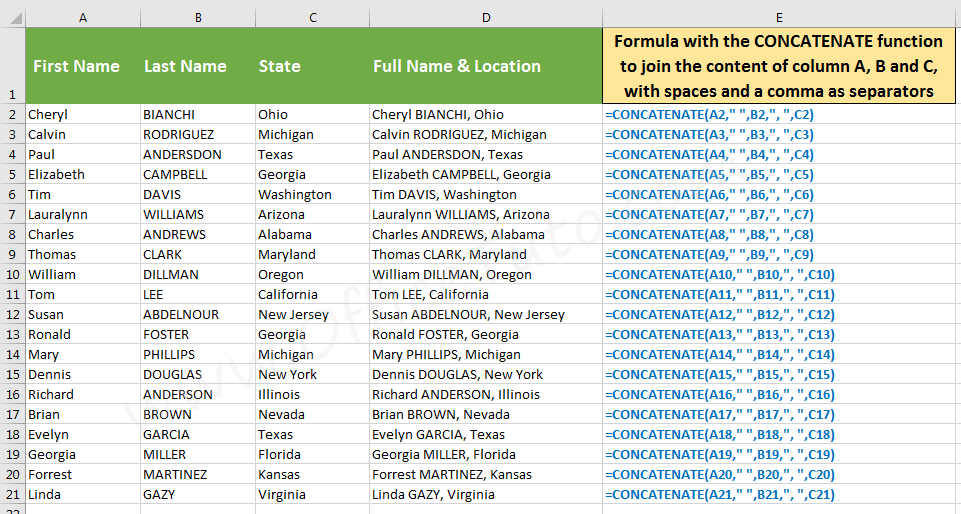
– Join 3 cells using CONCATENATE with space and comma separators

In this example, I use the CONCATENATE function to join first and last names, and their location (the state) from columns A, B, and C, and a space and a comma as separators; the result is in column D.

In the formula, the two spaces and the comma used as separators are put into double quotes; the syntax of the formula is: =CONCATENATE(first_cell,”space”,second_cell,”comma space”,third_cell)

The formula, for example from cell D2, is as follows: =CONCATENATE(A2,” “,B2,”, “,C2)

3- Join Excel cells with a separator using CONCAT function

The CONCAT function is available only in Excel 2019 and newer, or in Excel 365. Its syntax when inserting a separator is: =CONCAT(content1, “separator”, content2,…)

To join the content of multiple Excel cells with a separator between them (spacing, comma, semicolon, dash, colon, or any other text), using CONCAT function:

• In the result cell, type: =CONCAT(
• Click the first cell and type a comma
• Type the separator into double quotes
• Click on the second cell
• To join the 2 cells, press Enter. To join more:
• Type a comma. Then a separator in double quotes
• Click the next cell. And so on for the rest ones
• Finally, press Enter.

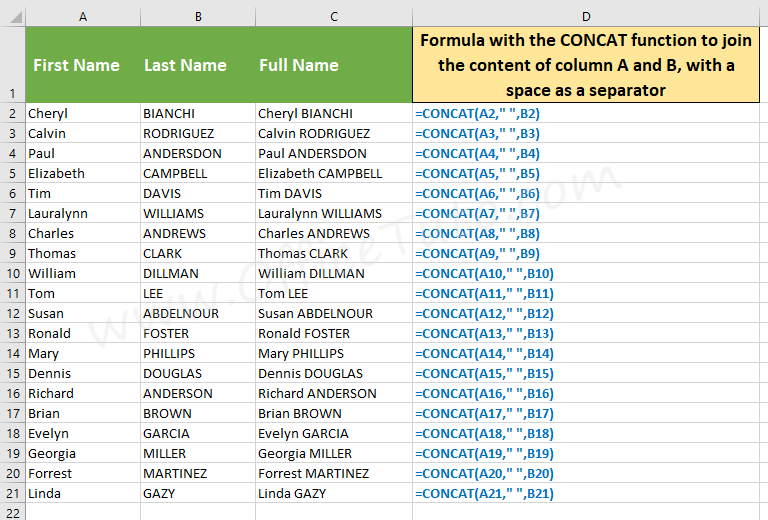
– Join first and last name with Excel CONCAT function

To illustrate how to join the content of two cells in Excel using the CONCAT function, with adding a separator between them, let’s take the following example where I want to join first and last names from columns A and B, with a space as a separator, and put the result in column C.

In the formula, the space used as a separator is put into double quotes; the syntax of the formula is: =CONCAT(first_cell,”space”,second_cell)

The formula, for example from cell C2, is as follows: =CONCAT(A2,” “,B2)

– Join 3 cells using CONCAT with space and comma separators

In this example, I use the CONCAT function to join first and last names, and their location (the state) from columns A, B, and C, and a space and a comma as separators; the result is in column D.

In the formula, the two spaces and the comma used as separators are put into double quotes; the syntax of the formula is: =CONCAT(first_cell,”space”,second_cell,”comma space”,third_cell)

The formula, for example from cell D2, is as follows: =CONCAT(A2,” “,B2,”, “,C2)

4- Join cells content with a separator using TEXTJOIN

The TEXTJOIN function is available only in Excel 2019 and newer, or in Excel 365. Its syntax when inserting a separator is: =TEXTJOIN(“delimiter”, ignore_empty_cells, content1, content2,…) or =TEXTJOIN(“delimiter”, ignore_empty_cells, first_cell:last_cell)

The formula =TEXTJOIN(“delimiter”, ignore_empty_cells, first_cell, second_cell,…) is for selecting individual cells (especially when not adjacent), whereas =TEXTJOIN(“delimiter”, ignore_empty_cells, first_cell:last_cell) is for when selecting a range of cells (requires adjacent cells).

• The delimiter is the separator to use to separate the content of the joined cells, and you’ll need to put it into double quotes. We’re using here one type of separators, but if we’re in the need of using different ones, we need to use a workaround as I will show you in the second example below (or use a different method or function!).
• The ignore_empty_cells is a boolean argument; so, it can be True (to not take into consideration the empty cells) or False (to join the empty cells). Can be useful when you have empty cells at the end of the range, otherwise choose either one.

– Join cells with one type of separators using TEXTJOIN

To join the content of Excel cells with one type of separator (spacing, comma, dash…) using TEXTJOIN function:

• In the result cell, type: =TEXTJOIN(
• Type the separator into two double quotes
• Type a comma, then True or False, then a comma
• If adjacent cells, select the range, then Enter.
• Otherwise, if non adjacent cells:
• Click the first cell and type a comma
• Click the next cell. And so on for the rest ones
• Finally, press Enter.

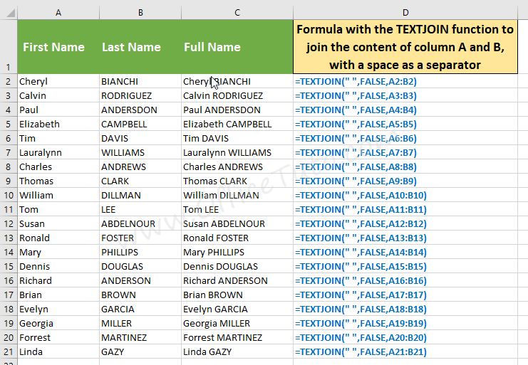
To illustrate how to join the content of two cells in Excel using the TEXTJOIN function, with adding a separator between them, let’s take the following example where I want to join first and last names from columns A and B, with a space as a separator, and put the result in column C.

In the formula, the space used as a separator is put into double quotes; the syntax of the formula is: =TEXTJOIN(“space”, ignore_empty_cells, first_cell:last_cell)

The formula, for example from cell C2, is as follows: =TEXTJOIN(” “, FALSE, A2:B2)

– Join cells with different separator types using TEXTJOIN

The Excel TEXTJOIN function is not really appropriate for joining the content of cells with different separator types, as it requires one single argument for the delimiter; but, there is a workaround if you really need to do this with TEXTJOIN (otherwise, the ampersand operator & or the CONCATENATE and CONCAT functions are much better appropriate).

To join the content of Excel cells with different separator types using TEXTJOIN function:

• In the result cell, type: =TEXTJOIN(“”,
• Type True or False, then a comma
• Click the first cell, then type a comma
• Type the separator in double quotes, then a comma
• Click the second cell, then type a comma
• Type the separator in double quotes, then a comma
• Click the next cell. And so on for the rest ones
• Finally, press Enter.

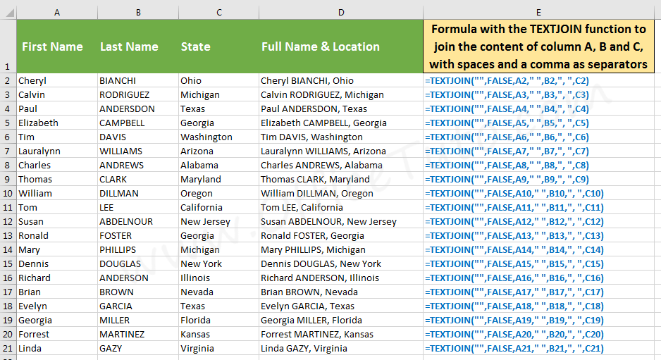
To illustrate how to join the content of three cells in Excel using the TEXTJOIN function, with adding different separators between them, let’s take the following example where I want to join first and last names, and their location (the state) from columns A, B, and C, and two spaces and a comma as separators; the result is in column D.

In the formula, the first opening and closing double quotes contain nothing (i.e. no separator); while the second and third ones contain respectively the space as first separator, then the comma and space as second separators. The syntax of the formula is: =TEXTJOIN(“”, False, first_cell, “space”, second_cell, “comma and space”, third_cell)

The formula, for example from cell D2, is as follows: TEXTJOIN(“”, FALSE, A2, ” “, B2, “, “, C2)

C/ Which one to use to join content in Excel: &, CONCATENATE, CONCAT, or TEXTJOIN

In all the above sections, I showed you that there were 4 ways to join the content of cells in Excel, be it with or without a separator; the ampersand operator &, and the functions CONCATENATE, CONCAT, and TEXTJOIN.

The problem that you may encounter is which one to use, depending on your situation!

In the following comparison table, I gathered the pros and cons of each method depending on some criteria, and included some formulas as examples, which will definitely guide you on which method to use when you want to join the content of the cells in Excel:

Comparison Table: & vs CONCATENATE vs CONCAT vs TEXTJOIN

Criteria	Ampersand operator &	CONCATENATE	CONCAT	TEXTJOIN
Excel Versions	All Excel versions	All Excel versions	Excel 2019 and newer, or Excel 365	Excel 2019 and newer, or Excel 365
When: No Separator, and with Adjacent Cells	Less appropriate (easiest method, but needs a manual selection of cells) Example: =A2&B2&C2&D2	Less appropriate (needs a manual selection of cells) Example: =CONCATENATE(A2,B2,C2,D2)	More appropriate (allows the selection of a range of cells with easy syntax) Example: =CONCAT(A2:D2)	Appropriate (complex syntax, but allows the selection of a range of cells) Example: =TEXTJOIN(“”,FALSE,A2:D2)
When: One Separator and Adjacent Cells The separator in the examples is the semi-colon symbol ;	Appropriate (easy syntax, but needs a manual selection of the cells and the repetition of the separator) Example: =A2&”;”B2&”;”C2&”;”&D2	Less appropriate (long syntax with no advantage: manual selection of cells, with repetition of separator) Example: =CONCATENATE(A2,”;”,B2,”;”,C2,”;”,D2)	Less appropriate (long syntax with no advantage: manual selection of cells, with repetition of separator) Example: =CONCAT(A2,”;”,B2,”;”,C2,”;”,D2)	More appropriate (the separator is typed one time only, and the selection of a range of cells is allowed) Example: =TEXTJOIN(“;”,FALSE,A2:D2)
When Different Separators Two separators are used in the examples: the semi-colon ; and the dash symbol –	More appropriate (easy syntax) Example: =A2&”;”B2&”-“C2&”-“&D2	Appropriate (long but easy syntax) Example: =CONCATENATE(A2,”;”,B2,”-“,C2,”-“,D2)	Appropriate (long but easy syntax) Example: =CONCAT(A2,”;”,B2,”-“,C2,”-“,D2)	Less appropriate (long and complex syntax with no advantage) Example: =TEXTJOIN(“”,FALSE,A2,”;”,B2,”-“,C2,”-“,D2)
When: Non-Adjacent Cells and No Separator	More appropriate (easy syntax) Example: =A2&C2&F2&G2	Appropriate (long but easy syntax) Example: =CONCATENATE(A2,C2,F2,G2)	Appropriate (long but easy syntax) Example: =CONCAT(A2,C2,F2,G2)	Less appropriate (long and complex syntax with no advantage) Example: =TEXTJOIN(“”,FALSE,A2,C2,F2,G2)
When: Non-Adjacent Cells and One Separator The separator in the examples is the semi-colon symbol ;	Appropriate (the separator needs to be typed as many times as the number of cells) Example: =A2&”;”&C2&”;”&F2&”;”&G2	Less appropriate (long syntax and the separator needs to be typed as many times as the number of cells) Example: =CONCATENATE(A2,”;”,C2,”;”,F2,”;”,G2)	Less appropriate (long syntax and the separator needs to be typed as many times as the number of cells) Example: =CONCAT(A2,”;”,C2,”;”,F2,”;”,G2)	More appropriate (the separator is typed one time only) Example: =TEXTJOIN(“;”,FALSE,A2,C2,F2,G2)
Selection of more than one range of cells	Not appropriate (you can’t select a range of cells)	Not appropriate (you can’t select a range of cells)	Not appropriate (you can use only one range of cells)	Appropriate (you can use more than one range of cells) Example: =TEXTJOIN(“”,FALSE,A2:D2,G2:K2)