How to Filter Data in Excel

Filters in Excel are easy to set up and offer a quick and easy way to view only pertinent data while hiding the other data on the spreadsheet.

Before we look at how to filter data in Excel, here are some tips on some recommended steps to do and points to check before filtering data, which will make the filter work better.

A/ Points to check before filtering data in Excel

There are 4 points that is recommended to check before filtering data in Excel:

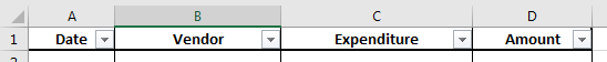
1- Set a header row for your data

The first row of the filter will always look for titles that provide information about each of the columns, therefore your spreadsheet should have a header row. This can be anywhere on the sheet, however, you can only create one filter per sheet, so often times this header row is in Row 1.

2- Freeze the header row of your data

Depending on the amount of data contained in your spreadsheet, it may be useful to freeze the header row, so it stays in the display even when scrolling down on the page.

If you don’t know how to freeze columns and rows, the How to Freeze Rows and Columns in Excel article will definitely help you.

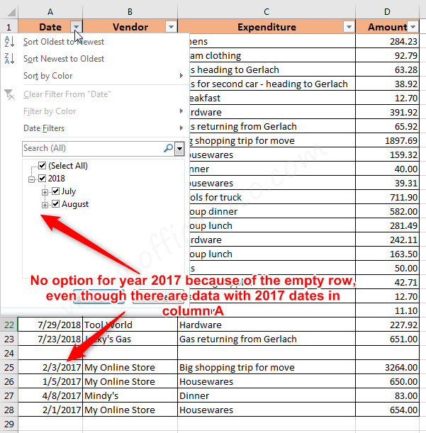
3- Remove blank rows from your data

Ideally, remove any complete blank rows separating the data which should be part of your filter, because they will not allow the cells below them to be chosen and displayed in the filter drop-down, as illustrated in the screenshot below.

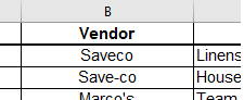
4- Ensure consistency of all your data

Review your data for consistency:

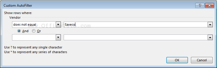
• When using filters, non-matching values are considered separately. Below is an example: “Saveco” and “Save-co” should be written the same way if they refer to the same thing.

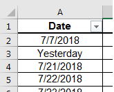
• Additionally, the format of data within each column should be the same. For example, if there is a cell formatted as Text within a list of dates, the filter options available will be affected.

With the above 4 guidelines in mind, you’re ready to filter your data.

B/ How to filter in Excel

To filter data from a range of cells in Excel:

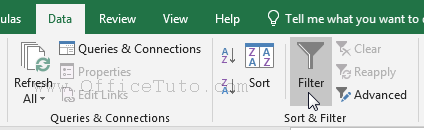
1. Click on a cell if you want all contiguous cells to be included, or select a part from the range if you want only a part to be included.
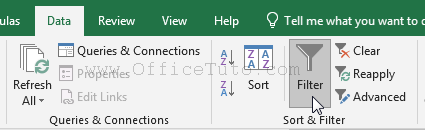
2. Go to the “Data” tab, then in the “Sort & Filter” group, click on “Filter”.

3. The “Filter column” arrow displays next to each column’s header.

4. Click on the filter arrow of the column you want to filter.
5. Check the items you want to be filtered and displayed, and uncheck the ones you don’t want.
6. Or, use the options “Filter by Color” or “Text Filters/Date Filters/Number Filters”.

7. Once you have selected the data you want to filter, click OK to view the filter on your spreadsheet.
8. Excel immediately filters data based on the chosen criterion and changes the look of the “Filter arrow” on the filtered column’s header to indicate that a filter is applied on it.

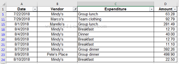
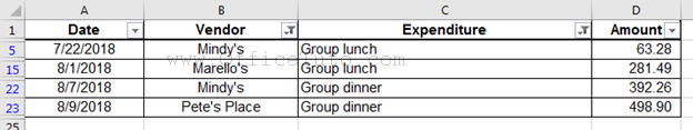
Note that the row headers are now blue, with gaps between rows numbers, which indicates that not all rows are now being displayed on the sheet, only the filtered ones.

Note: How can you verify if a filter is actually applied and on which column? You can do this by checking 4 things:

• There are arrows on the columns labels.
• The “Filter” command of “Data” tab is highlighted.
• Row headers are blue.
• There are numbering gaps between the rows headings.

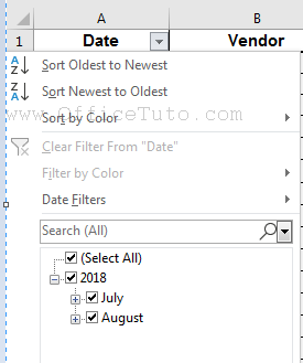
Multiple columns can be filtered at the same time. In the below example, we are showing only certain Vendors (Column B) where the Expenditure column (Column C) also only displays certain values.

Note: Options in the filter dropdown will vary depending on the data type in the column being filtered (Text Filters, Date Filters, or Number Filters):

– When filtering on a Date formatted column: Sort options allow to “sort from oldest to newest” and “from newest to oldest” and the checkboxes are organized into a tree allowing more specification in the dates or group of dates (by month and year).

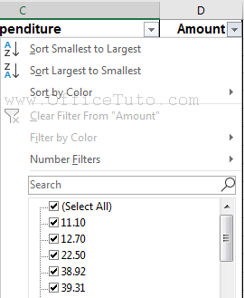
– When filtering on a Number formatted column: Sort options allow to “sort from smallest to largest” and “from largest to smallest” and the checkboxes are ordered from smallest to largest by default to make scrolling through the list more efficient.

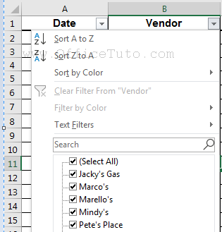
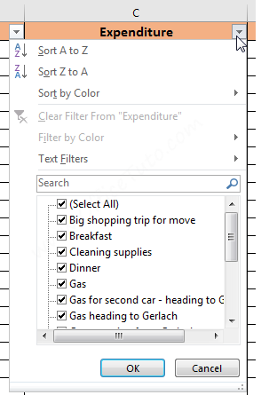
– When filtering on a Text formatted column: Sort options allow to “sort A to Z” and “Z to A” and the checkboxes are alphabetically ordered to make scrolling through the list easier and more efficient.

– Options provided in the filter dropdown (Text formatted column as an example)

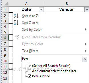
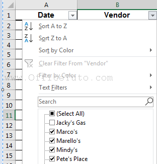
The filter dropdown menu offers many options for filtering the data shown, and it also allows the data to be sorted in various ways (see the screenshot to the right); I’m taking here a text formatted column as an example:

• Sort alphabetically, options for “A to Z” and “Z to A”.
• Sort by color.
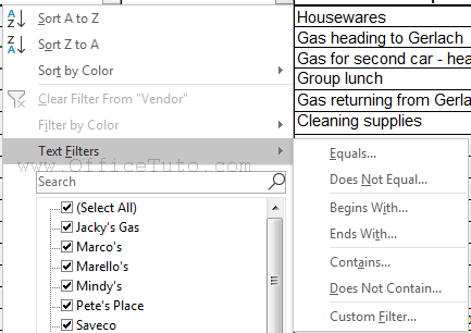
• Text filters:
  • Text equals…
  • Text does not equal…
  • Text begins with…
  • Text ends with…
  • Text contains…
  • Text does not contain…
  • Custom filter…

The “Sort by color” and “Text Filters” options bring up the Custom AutoFilter dialog box, which lets you select one or more criteria to display.

• Below the “Text Filters” option, you have the “Search” area which allows you to type part or all of the data within the fields you want to filter and displays the results in the list below.

• Checkboxes allow you to select or unselect certain data values, or select/unselect all the values.

C/ How to clear a filter in Excel

Clearing an Excel filter is to cancel it and display all data, with no filtered items, without removing the filter: the filter is still on and the arrows are still available in the columns headers so you can use them whenever you want. To clear a filter, this one needs to be already applied and some data filtered.

Once again, clearing a filter in Excel is not removing it!

You can clear all the filters of an Excel spreadsheet, or only the filter of a specific column, as I show you below:

– Clear the filter of all columns in an Excel spreadsheet

To clear the filter of all the columns in an Excel spreadsheet:

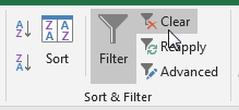
1. Go to the “Data” tab.
2. In the “Sort & Filter” group, click on “Clear”
3. All data will be shown, with no filtered ones.

– Clear the filter of a specific column of an Excel sheet

To clear the filter of a specific Excel column to display all its rows that can be shown and let the other columns filtered:

1. Click the filter arrow on the column header.
2. Choose the option “Clear Filter From…”.
3. The filter of this only column is cleared.

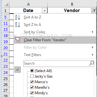
Of course, not all rows of the unfiltered column can be shown, as this depends on the filters applied to the other columns.

D/ How to remove the filter from the spreadsheet

If you don’t want the filter anymore on your spreadsheet, you can remove it altogether.

To remove the filter from an Excel spreadsheet:

1. Go to the “Data” tab.
2. In the “Sort & Filter” group, click on “Filter” to unselect it.
3. The filter is deactivated: no arrows on columns headers and all rows are shown.

E/ Conclusion

I hope you’ll find this tutorial on how to filter in Excel very useful; the AutoFilter options described along all this article should allow you to filter and review specific data on your spreadsheet with many different options.

For more complicated filtering, consider using other Excel features, like the Advanced Filter or Pivot Table.

- "Learn Excel: For Beginners" Series Navigation:

<< 8: How to Freeze Rows and Columns in Excel