Anyone who uses Microsoft applications would agree that Excel formulas and functions are one of the most important features offered by these applications.
Therefore, I will detail in this Excel tutorial everything you need to learn about Microsoft Excel formulas and functions: how to create Excel formulas, how to use them along with functions, how to edit them, how to copy them to a column or row, and how to show or trace the cells containing them.
1- What are Excel Formulas and Functions
Formulas and functions are a key feature in the daily use of Excel, whether for experienced users or even Excel beginners.
You can think of Excel formulas as usual mathematical formulas. They have operators and operands, and they allow to perform calculations.
They can either be simple, with just operands and operators, or include predefined functions already available in Excel to offer more complexity:
– Examples of simple Excel formulas:
- =165+203
- =A2-64.58
- =A3+B3
- =(A3*B3)/C3
– Examples of Excel formulas with functions:
- =SUM(B2:B15)
- =PRODUCT(D8:H8)
- =AVERAGE(C3:C15)
The functions shown in these formulas are SUM(), PRODUCT(), and AVERAGE(). Which is into parentheses are the ranges of cells indicated by a colon mark.
I will explain all of that in the following sections.
Now, before diving into more details about Excel formulas and functions, let’s first start with some guidelines that will allow you to better benefit from this tutorial and to make good use of Excel formulas in the future.
a- Guidelines about Excel formulas
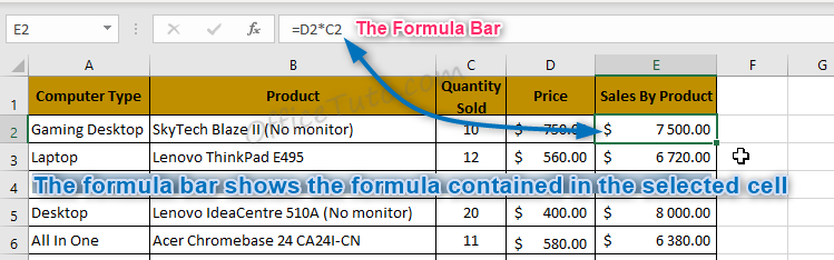
- Excel formulas can be entered in the cell itself or in the “Formula Bar” (after selecting the result cell).

- All Excel formulas start with an equal sign (=).
It is automatically inserted when you create an Excel formula by inserting a function from the ribbon; otherwise, if you manually create a formula, you should enter the equal sign yourself.
- Cell References:
A cell in Excel is referenced by its column and row; meaning we can’t refer to a cell in Excel without its reference, unless we gave it a name. Cell references are extremely important in Excel formulas.
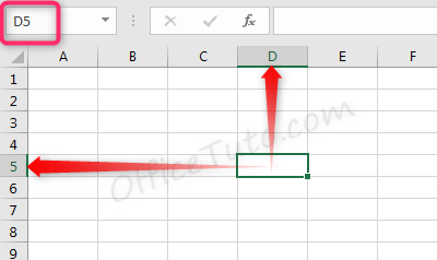
For example, in the illustration below, I’m selecting the cell that intersects column D and row 5. So, the reference of my cell is D5, as you can see in the “Name box“.

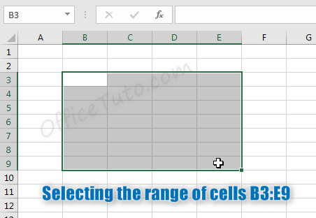
- The colon mark (:) indicates a range of cells. A range of cells is referenced by its first and last cell references, separated by a colon.
e.g. (B3:E9) means the range of cells from B3 to E9.
- You can validate your formula by either pressing Enter on the keyboard or clicking the “checkmark” on the left of the “Formula Bar”.
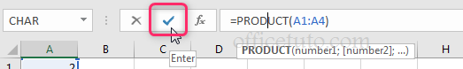
As you may experience, it’s much better to directly press Enter after finishing your formula than to click with the mouse!
- Simple Excel formulas can contain operators (+;-;*;/;^), numbers (12; 1689.56; etc), and cells references (A3; B68; etc);
In addition to these elements, complex Excel formulas can contain functions, ranges of cells (SUM(A2:A15); PRODUCT(B3:F17); etc), and arguments.
More on that right below…
b- Simple Excel formulas
Simple Excel formulas are simple formulas that contain just operands and operators.
For example: in the formula =A2+B2, the operands are A2 and B2, and the operator is the + sign.
In a basic Excel formula, an operand is a cell reference or a number.
To better understand what are really Excel formulas in their simple form, let’s consider the range A2:C7 (from the cell A2 to C7) and provide some examples to perform calculations with the help of simple Excel formulas.
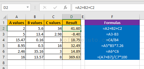
Note: The formulas are of course to be entered into the cells results that you designate yourself; in my following examples, the formulas were entered in the respective cells of D column (see the screenshot below).
And of course, ignore column F in my screenshot; it is there just for explanatory purposes.
– Examples of simple Excel formulas:
- Addition formula:
=A2+B2+C2 - Subtraction formula:
=A3-B3 - Division formula:
=C4/B4 - Multiplication formula:
=A5*B5*7.26 - Power formula:
=A6^C6 - Mixed formula:
=(A7+B7)/C7*100
In all these simple Excel formulas, we have an equal sign (as all Excel formulas), operators (mathematical symbols), and operands (cells references and constants).
For example:
- In the first formula
=A2+B2+C2: the operator is the plus symbol (+) for addition, and the operands are the cells references A2, B2, and C2. - In the last formula
=(A7+B7)/C7*100: the operators are the plus symbol (+) for addition, the slash symbol for division, and the asterisk symbol for multiplication; and the operands are the cells references A7, B7, and C7, and the constant 100.
c- Excel functions
Built-in functions can be of great help in your formulas. They provide a very useful way to perform calculations, and each one of them has its own particular layout and arguments, which is called “Syntax“.
A general syntax for Excel formulas with functions is like this:
=FUNCTION_NAME(arguments_if_any)
with 3 forms:
- Function with no arguments:
=FUNCTION_NAME() - Function with one argument:
=FUNCTION_NAME(one_argument) - Function with multiple arguments:
=FUNCTION_NAME(argument1, argument2, argument3...)
Arguments of a function are any data this function would need to perform its task of calculation; and depending on the function used and the formula, these arguments could be a cell reference, a range of cells, a number, a text, or even another function.
Function arguments are always contained within parentheses and separated from each other with a comma.
As we have done with simple formulas, and to better understand what are really Excel formulas with functions, let’s consider the range A2:C5 (from the cell A2 to C5) and provide some examples to perform calculations with the help of some Excel formulas with functions:
– Examples of Excel formulas with functions:
- Function with no arguments:
- Function PI that returns the value of the mathematical constant Pi:
=PI() - Function TODAY that returns today’s date:
=TODAY()
- Function PI that returns the value of the mathematical constant Pi:
- Function with one argument:
- Summation formula using SUM function:
=SUM(A2:A5) - Average calculation formula using AVERAGE function:
=AVERAGE(A2:A5) - Formula of finding the greatest value of a range using MAX function:
=MAX(A2:A5)
- Summation formula using SUM function:
- Function with multiple arguments:
- Summation formula of 2 ranges of cells using SUM function:
=SUM(A2:A5, C2:C5) - Summation formula of a range of cells based on a condition, using SUMIF:
=SUMIF(A2:A5, E2, C2:C5)
- Summation formula of 2 ranges of cells using SUM function:
2- Where and how to create an Excel formula
Regarding the creation of a formula in Excel, I will discuss the 2 aspects of it: WHERE to create the formula, and HOW to do it.
a- Where to create an Excel formula
There are 2 placements where you can create your formula :
- Inside the output cell itself (the cell where you want the result to be), by clicking on it.
- In the Formula bar after selecting/clicking the output cell.
b- How to create an Excel formula
There are 3 ways of creating a formula in Excel.
You create a formula in Excel by:
- writing the formula in the cell or the Formula bar
- clicking on the fx button (Insert Function)
- or by using the Formulas tab of the ribbon
Let’s detail, in the following sections, all these three methods of creating a formula in Excel.
b1- Writing the formula in the output cell or Formula bar
This method can be used for ALL Excel formulas (formulas with or without functions).
So, to manually create a formula in Excel:
- Click on the result cell.
- or select it and click in the Formula bar.
- Write the formula following its syntax.
- Press Enter key of the keyboard.
As an example, let us consider the SUM function:
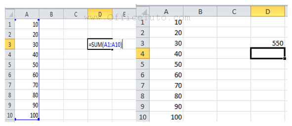
If I need to get the summation of values of all the cells from A1 to A10, I just have to write the following formula in the cell where I need to output the result:
=SUM(A1:A10)
And hit Enter.
That’s it; so simple!
In the following screenshot, I wrote my formula in the cell D3.
b2- Create a formula in Excel using the fx button
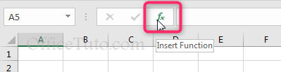
This method is to be used for Excel formulas with functions.
You should first select the output cell, then click on the “Insert Function” button (the fx button next to the Formula bar); Excel will then display the “Insert Function” dialog box (see the image below), where you can select or search for the function you need.
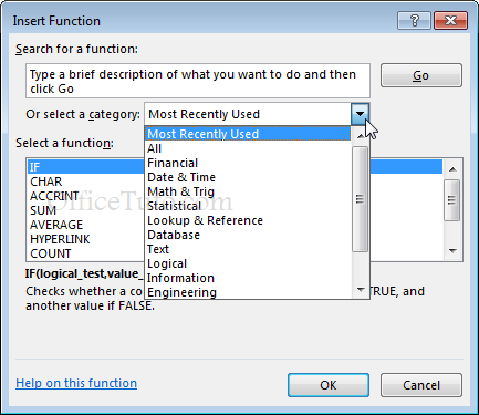
Once you select a function, you’ll get, below the functions list, the syntax of this function and a description of what it does; see the screenshot above.
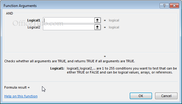
When you click OK, Excel will display another dialog box called “Function Arguments” where you can enter the arguments (if any) for the function in the required fields. In the example illustrated below, I chose the “IF function”.
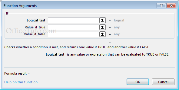
Information in the lower section of this dialog box explains what this function is for (purpose of the function) and what information is needed to perform it (Arguments definition). Click in each of the value boxes and read the information about it.
I won’t go further here as there are lots of functions in Excel and each function has its own syntax, which will go beyond the scope of this general and introductory article; but you’ll find more detailed explanations in other Excel tutorials on formulas and functions.
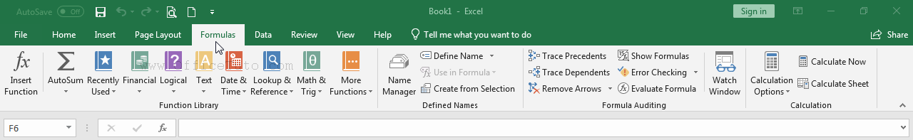
b3- Create a formula in Excel using the Formulas tab
This method too is to be used for Excel formulas with functions.
As you can see from the above image, Excel makes it easy for users to find the right functions by grouping them into some categories.
Excel has function groups like financial, date time, math and trigonometry, statistical, lookup, database, text, logical, information, engineering and many more.
Here again, once you choose a function from a category (except the “AutoSum” drop-down list), Excel will display the “Function Arguments” where you can enter the arguments (if any) for the function in the required fields.
As explained in the previous section “Create a formula in Excel using the fx button”, the “Function Arguments” dialog box displays in its bottom a description of the function’s purpose and a definition of the arguments, if any.
As for the “AutoSum” category in the “Formulas” tab of the ribbon, Excel will directly insert the function in the output cell waiting for you to manually enter its arguments.
3- How to edit an Excel formula
Sometimes we may want to modify an existing formula. This is easy as you don’t have to delete it and create a new version of it.
So, to edit a formula in Excel:
- Click the cell with the formula, then the “Formula bar”
- or double-click the cell with the formula.
- A border will appear around referenced cells.
- Modify the part of the formula you need.
- When you’re finished, press Enter
- or click the checkmark in the formula bar.
- The formula will be updated.
- And the new value will display in the cell.
– How to cancel changes while editing a formula
While editing your formula, you may make some accidental or unwanted changes to it; if this occurs, you can just press Esc key of your keyboard to undo them.
4- How to copy an Excel formula to a column or row
When you create a formula in an Excel cell and need the same for other cells of your range, you won’t recreate your formula in all the range cells, one by one. You just need to copy or extend it to the rest of your range following the methods I will explain below.
There are 3 ways to copy or extend an Excel formula to a column or row:
- Using the fill handle.
- Using the fill command of the ribbon.
- Or using a keyboard shortcut.
a- Copy Excel formula using the fill handle
To copy or extend an Excel formula to a column or row using the fill handle, just:
- Click the cell containing your formula.
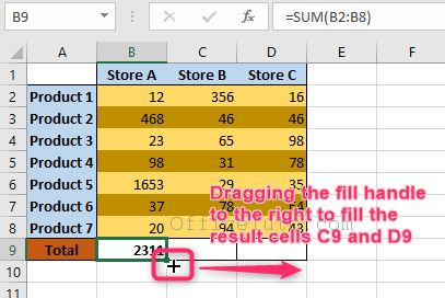
- Drag the fill handle to copy the formula to the desired range of cells in a row or column.
- Or double-click the fill handle and Excel will automatically fill the remaining cells of the range, provided there are no merged cells in the way.
The fill handle is the small square in the bottom-right of a selected cell; see the screenshot below.
b- Copy Excel formula using the fill command of the ribbon
To copy or extend an Excel formula to a column or row using the “Fill” command of the ribbon:
- Enter the formula in the first cell of the range
- Select the whole range, including the first cell with formula
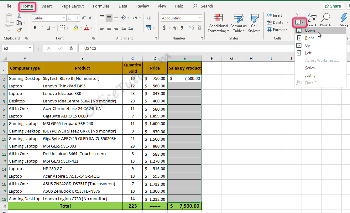
- Go to the “Home” tab of the ribbon
- Go to the group of commands “Editing”
- Click on the “Fill” drop-down list
- Choose an option: “Down”, “Right”, “Up”, or “Left”.
Meaning, if you want to copy a formula across a column, choose “Down” or “Up” depending on the location of the cell you enter the formula in; the first cell of the range, or the last one.
Similarly, if you want to copy a formula across a row, choose “Right” or “Left” depending on the location of the cell you enter the formula in; the first cell of the range, or the last one.
c- A shortcut to copy Excel formula
Dragging the fill handle across an Excel column or row with too many cells would be a bit of a hassle.
If this is your case, you would rather like to use a keyboard shortcut to quickly get the job done, wouldn’t you?
Fortunately, you can really do that in Excel.
So, To copy or extend an Excel formula to a column or row using a keyboard shortcut:
- Select the whole range of cells in your column or row where you want to copy the formula to
- Enter your formula (if you have previously entered it before selecting the cells, just enter it again)
- Press the keys combination “Ctrl + Enter” (hold down the Ctrl key and press Enter of your keyboard).
- Excel automatically fills the other cells of the range with the formula, respecting of course the cells references.
5- Cell references in Excel
In this section, I will tell you what are cell references in Excel, will define and compare their three types with examples (relative, absolute, and mixed references), and show you how to refer to another spreadsheet of the same workbook.
a- What are cell references in Excel
A cell reference in Excel indicates the position of the cell in the sheet by its column and row; e.g. the reference of the cell intersecting column B and row 2 is B2. A range of cells is referenced by its first and last cell references, separated by a colon; e.g. the range of cells from A3 to F7 is referenced by A3:F7. We use references to the cells or ranges in the formulas.
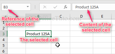
To better illustrate the cell reference, I give you an example in the screenshot below, where I’m selecting the cell that intersects column D and row 5. So, the reference of the selected cell is D5, as you can see in the “Name Box”.
The cell reference doesn’t of course reflect the content of the cell, which is displayed in the cell itself and in the Formula bar, as illustrated below.
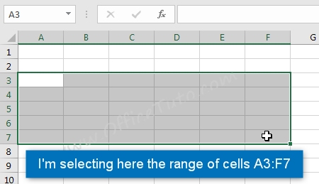
In the screenshot below, I’m selecting the range of cells from A3 to F7; so, the reference to this range is A3:F7.
b- Types of cell references: relative, absolute, and mixed
I couldn’t talk about different types of cell references (relative, absolute, and mixed references) earlier in this Excel tutorial, as this would make no sense if you don’t already know why and how to copy an Excel formula; the absolute or mixed references of cells may be used only when copying an Excel formula to another cell or through a range of cells.
b1- Relative references in Excel
By default, a cell reference in Excel is relative; meaning, it depends on the position of the cell containing the formula, and of course on the cells referenced in it. So, if you copy the formula to another cell, this formula will adjust its references itself.
We already saw that in the previous section when copying an Excel formula through a column or row, but let’s see it again in an example:
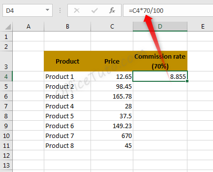
Suppose that I have the following data of prices of products, and I want to calculate the commission rate of 70% for each price:
To calculate it for the price in the cell C4, I type in the result cell D4, the following formula:
=C4*70/100
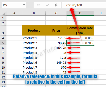
Then, I want to copy the formula to the cells of the range D5:D11.
Let’s start by doing it just to the cell D5; I copy the formula from the cell D4 and paste it in the cell D5, and Excel changes the pasted formula to the following:
=C5*70/100
Which is great as that’s what I want really to have!
How is that?
Cell references are relative by default in Excel.
In my example, Excel knows from the formula in the first cell D4 that it uses a reference to the first cell on its left; so, when I paste the formula in the new cell D5, Excel considers the position of this new cell and accordingly changes the reference within it to match the cell on the left of D5, which is C5.
Let’s now check the other types of cell references, absolute and mixed ones.
b2- Absolute references in Excel
Unlike relative references, absolute references in Excel don’t change with the position of the cell containing the formula. They won’t change when you copy their formula to another cell or through a range of cells. To get an absolute reference, use the $ symbol before the references to the column and to the row of the cell.
For example, to use absolute references in the Excel formula =C4, I should use two $ symbols; one, before the reference of the column, and one before the reference of the row: =$C$4.
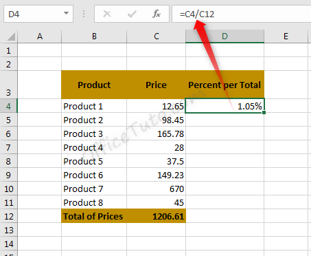
Let’s take the following concrete example, where I want to calculate the percent of each price per the total.
I use the formula =C4/C12 in the result cell D4, as illustrated below.
And I want now to copy the formula to the cells of the range D5:D11. When I copy it to the cell D5, I get an error of “dividing by zero or by an empty cell”; see the following screenshot:
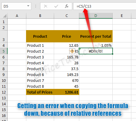
This isn’t an error from Excel, but instead from my logic. When I copy the formula down, Excel just adjusts the relative references in it which leads to an error since the cell C13 doesn’t have any content in it. My initial intent was to divide all the cells by the same cell C12 containing the total of the prices. To get this right while copying the formula to other cells, I should fix the reference to the cell C12 in the formula with the use of the $ symbol.
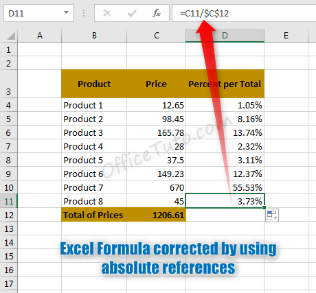
The formula in the first cell D4 should then be: =C5/$C$12
Here is the result after editing the formula in the cell D4 with absolute references and copying it through the range of cells D5:D11.
b3- Mixed references in Excel
As their name suggests, mixed references are a mix of relative and absolute references: they either contain a relative reference to column and absolute reference to row, or relative reference to row and absolute reference to column. So, they contain one $ symbol (before the column reference or the row reference).
For example:
If the formula =C4 has relative references, and the formula =$C$4 has absolute references, the formula with mixed references would be =C$4 or =$C4:
- With the formula
=C$4, we are fixing the reference to the row 4 and the column reference will change while copying the formula (row reference is absolute and column reference is relative). - With the formula
=$C4, we are fixing the reference to the column C and the row reference will change while copying the formula (column reference is absolute and row reference is relative).
c- How to quickly apply a relative, absolute, or mixed reference in Excel
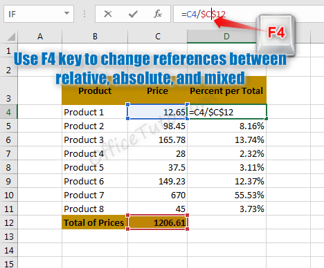
You know now that to indicate an absolute or mixed reference in an Excel formula, you should use the $ symbol. But, you need to know that you can have the same result without typing it yourself in the formula; just use the F4 key of your keyboard.
So, to quickly switch between relative, absolute and mixed references in an Excel formula, click in the “Formula Bar” on the reference part of your formula you want to change, and press the F4 key of your keyboard to change the reference; press it again and again until you get what you want.
d- Reference to another Excel sheet of the same workbook
I deliberately let this section until this stage, giving you enough time to well assimilate the basic concepts of Excel formulas and functions.
You may sometimes need to refer to some values from another sheet of the same workbook (refer to a cell or a range of cells); here is how to do that:
To refer to another Excel sheet of the same workbook, use the name of the sheet with an exclamation point before the cell or the range of cells reference. For example: Sheet1!A2 (for the cell A2 of the spreadsheet named “Sheet1”), or 2019!B3:B27 (for the range of cells B3:B27 of the spreadsheet called “2019”).
Let’s take the following example where we have two Excel sheets: “Summary” and “Prices”.
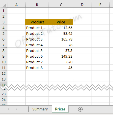
- Refer to a cell from another sheet of the same workbook
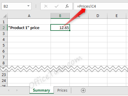
In the “Summary” sheet, I want to have the value of, let’s say, the price of “Product 1”.
So, in my result cell in the “Summary” sheet, which is the cell B2 (see the following screenshot), I will enter this formula:
=Prices!C4
Meaning, I’m getting the value of the cell C4 from the sheet “Prices”, into my cell B2 of the “Summary” sheet.
Note: Instead of manually writing this formula, I could also just typed the equal sign, then clicked on the “Prices” sheet, clicked on the C4 cell of this sheet, and pressed Enter.
- Refer to a range of cells from another sheet of the same workbook
Let’s now see another case from the same example where I will use a function in my formula, applied to a range of cells:
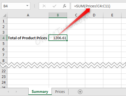
For example, the Excel SUM function to get, into my “Summary” sheet, the sum of the range of cells C4:C11 from “Prices” sheet.
So, in my result cell in the “Summary” sheet (cell B4), I will enter the following formula:
=SUM(Prices!C4:C11)
Meaning, I’m asking Excel to calculate the sum of the range of cells C4:C11 from “Prices” sheet and put the result into my result cell (B4) of the “Summary” sheet.
Note: Instead of manually writing this formula, I could also just typed =SUM(, then clicked on the “Prices” sheet, selected the range of cells C4 through C11 of this sheet, and pressed Enter.
Note about the name of the sheet in the formula:
Get in mind that the name of the sheet in an Excel formula is a text; so, for your formula to be accepted by Excel, the name of the sheet used in should be of one word; otherwise if the name contain a space or a number, you should surround it by an apostrophe (‘).
Note that for a name as a number or containing a number, even if you don’t use the apostrophes, Excel will correct your formula and add them automatically!
Examples:
- If my “Prices” sheet was called “Prices of Products”, the above formulas should be:
='Prices of Products'!C4
And,
=SUM('Prices of Products'!C4:C11)
- If my “Prices” sheet was called “Prices2019”, the above formulas should be:
='Prices2019'!C4
And,
=SUM('Prices2019'!C4:C11)
- If my “Prices” sheet was called “2019”, the above formulas should be:
='2019'!C4
And,
=SUM('2019'!C4:C11)
6- How to show formulas in Excel
In this section, I will show you how to display the formula of a cell, as well as all the formulas of a sheet, how to highlight all cells containing a formula, and how to trace the cells used in a formula.
a- How to display the formula of a cell in Excel
To view the formula of a single cell containing an Excel formula, you just need to select this cell (i.e. click on it), then view its formula in the “Formula Bar”.
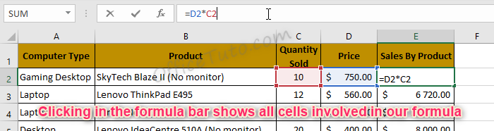
If you want to display the formula in the cell itself (in addition of course to the Formula bar) with highlighting all the cells involved in it, just double-click on the cell, or select the cell and click in the “Formula Bar”.
Excel will display the formula in the cell itself and highlight all the cells involved in the formula with different colors, so you can notice them easily.
You can also use a keyboard shortcut to show the formula of a cell and highlight all other involved cells: Click the cell containing the formula and press F2 key of your keyboard.
To get back to the values display, press Esc (Escape key) of your keyboard.
b- How to display all formulas of an Excel sheet
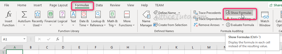
To display all formulas of an Excel sheet, you can use the ribbon by going to the “Formulas” tab and clicking on the “Show Formulas” command from the “Formula Auditing” group, or you can also use the keyboard shortcut Ctrl + ‘.
Let’s detail more these two methods in the following:
b1- Display all formulas in Excel using the ribbon
To display all formulas of an Excel sheet using the ribbon, go to the “Formulas” tab of the ribbon, then in the “Formula Auditing” group of commands, click on “Show Formulas”. Excel shows formulas instead of calculated values in all the cells containing formulas.
For example, we have some formulas in the following Excel sheet that we want to display:
Here is the Excel sheet before:

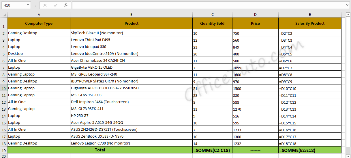
Here is the Excel sheet after showing all its formulas:
b2- Display all formulas in Excel with a shortcut
To display all formulas of an Excel sheet using the keyboard, just use the Ctrl + ' shortcut. Meaning, you hold down the Ctrl key and press the single quotation mark of your keyboard.
This shortcut is a toggle one; so, to get back to the values instead of the formulas, just use it again.
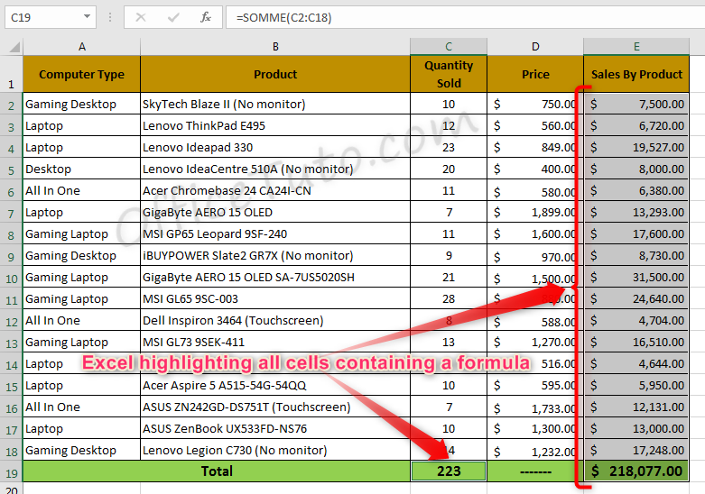
c- How to highlight all cells of an Excel sheet containing a formula
Sometimes, you would need to know which cells in your Excel sheet are containing a formula, without the need to show all these formulas.
The solution is to let Excel highlight them for you.
So, to highlight all cells of an Excel sheet containing a formula:
- Start by pressing the F5 key of your keyboard.
- Excel opens the “Go to” dialog box.
- Click on “Special” button.
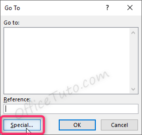
- Excel opens the “Go To Special” dialog box.
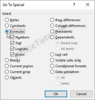
- Select “Formulas” and click “OK“.
Here is how does this look in my example of Excel sheet:
d- How to trace the cells used by an Excel formula
Another feature that allows you to understand the behavior of an Excel formula in a cell and visually discern all cells involved in it, is to trace the precedents and the dependents of this cell.
You’ll find this feature in the “Formulas” tab of Excel ribbon, within the “Formula Auditing” group of commands.
Tracing the precedents of a cell containing an Excel formula is finding the cells used in the formula; i.e. affecting the result.
On the other hand, tracing the dependents of a cell is finding the cells using this particular cell in a formula; i.e. finding the cells affected by our selected cell.
Let’s put this into practice in the following sections.
d1- Trace the precedents of a cell containing an Excel formula
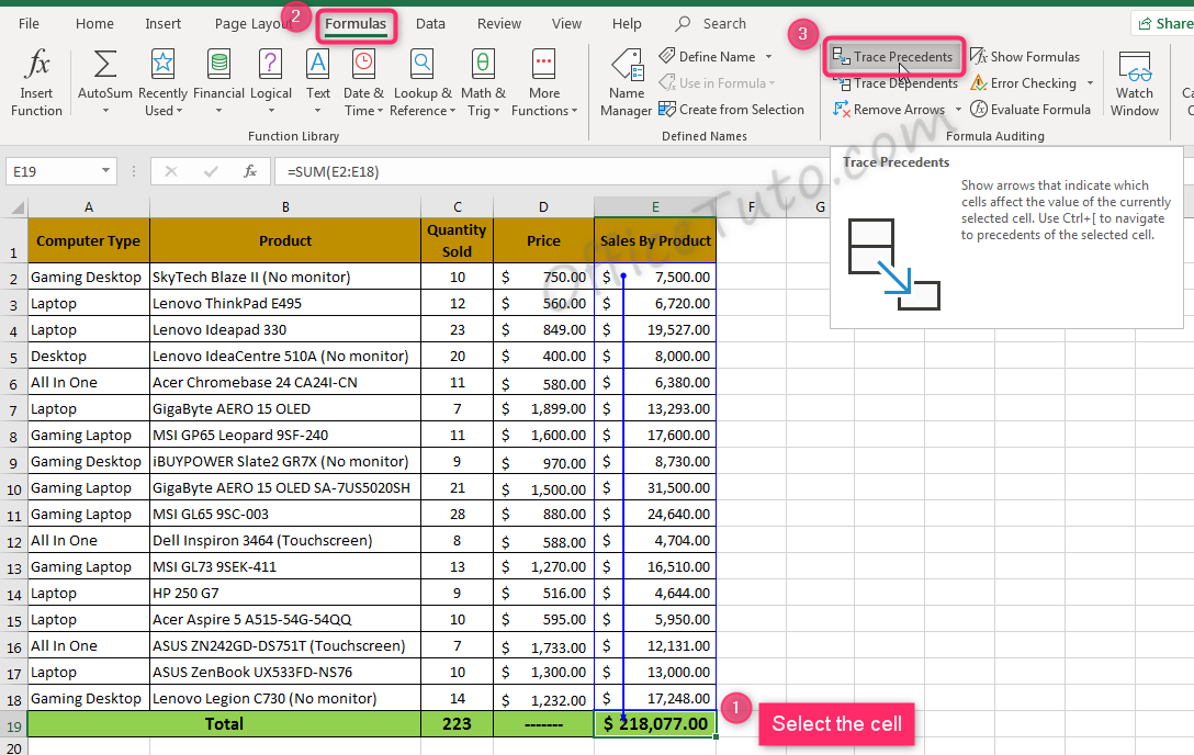
To trace the precedents of an Excel cell containing a formula:
- Select the cell containing the formula.
- Go to the “Formulas” tab of the ribbon.
- Then, go to the “Formula Auditing” group.
- Click on the “Trace Precedents” command.
- Excel shows with arrows the process of the formula.
- Click again on the “Trace precedents” command.
- Excel shows the second level of precedents, if any.
- And so on.
Let’s see all of this in an example:
In the example illustrated below, I want to trace the precedents of the cell E19 containing the formula =SUM(E2:E18).
So, I select this cell E19 and click in the “Formulas” tab on the “Trace Precedents” command. Excel draws an arrow indicating the process of my formula, from the range of cells E2:E18 to the result cell E19.
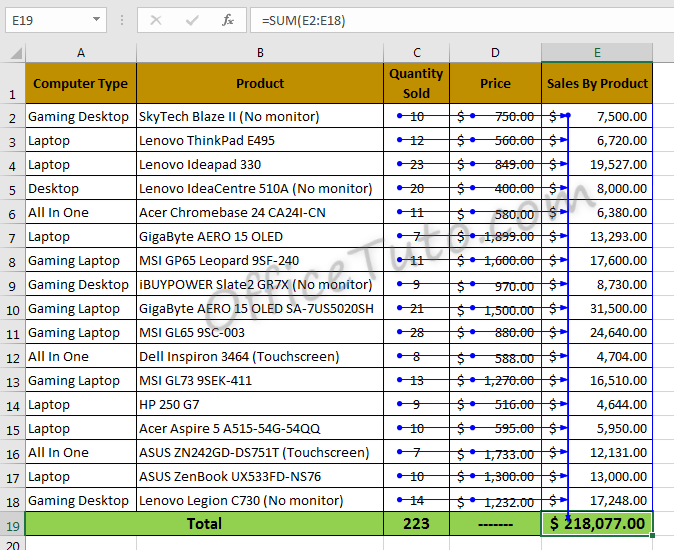
Clicking one time again on the “Trace Precedents” command gets me to the second level and reveals the precedents of the range of cells E2:E18 itself.
See the result in my example:
To cancel the effect of the “Trace Precedents” command and remove the arrows, go to the d3 section on removing the arrows of tracing precedents and dependents of a cell with formula.
d2- Trace the dependents of a cell contributing to an Excel formula
To trace the dependents of an Excel cell contributing to a formula or formulas:
- Select the desired cell.
- Go to the “Formulas” tab of the ribbon.
- Then, go to the “Formula Auditing” group.
- Click on the “Trace Dependents” command.
- Excel shows with arrows how the cell contributes to the formula(s).
Let’s see all of this in an example:
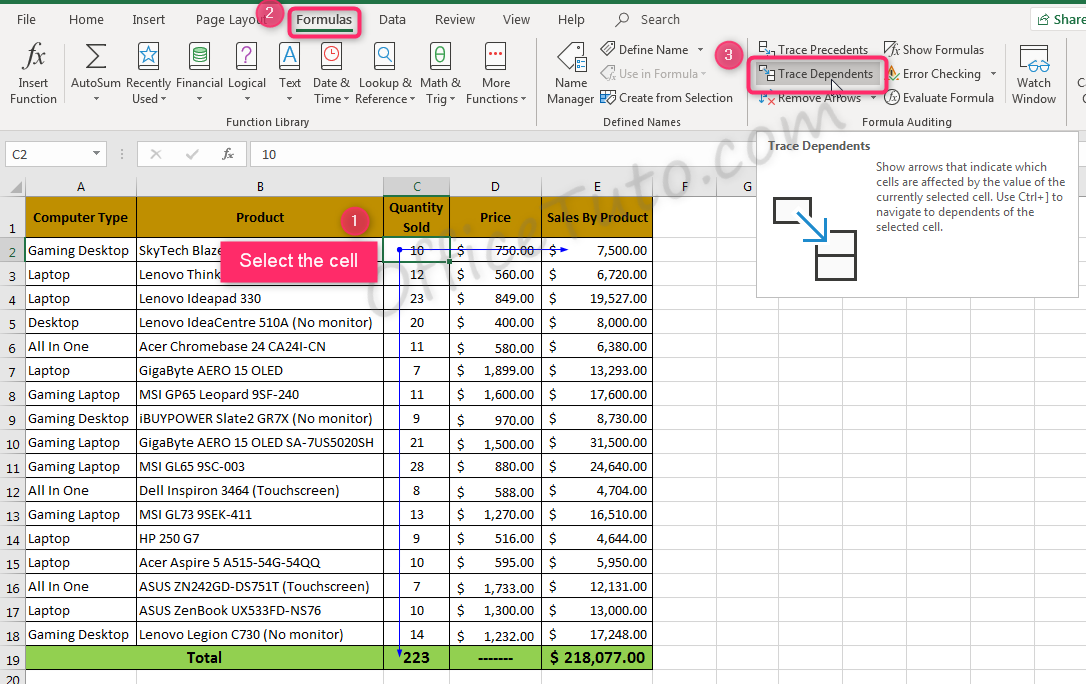
In the example illustrated right below, I will trace the dependents of the cell C2 for example, to see which formulas this cell is contributing to.
So, I select the cell C2 and click in the “Formulas” tab on the “Trace Dependents” command.
Excel draws two arrows from my cell C2 to the cell E2 and the cell C19, indicating that C2 is used in the formula contained in E2 (which is =C2*D2), as well as in the other formula contained in C19 (which is =SUM(C2:C18)).
To cancel the effect of the “Trace Dependents” command and remove the arrows, see the following section.
d3- How to remove the arrows of tracing precedents and dependents of a cell
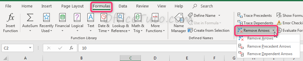
To cancel the effect of the “Trace Precedents” and/or the “Trace Dependents” commands, meaning to remove the arrows they drew on your data:
- Go the “Formula” tab of the ribbon,
- Go to “Formula Auditing” group of commands,
- To remove all arrows, click on “Remove Arrows”.
- To remove only one type of arrows, expand the drop-down list and choose an option.

Jeff Golden is an experienced IT specialist and web publisher that has worked in the IT industry since 2010, with a focus on Office applications.
On this website, Jeff shares his insights and expertise on the different Office applications, especially Word and Excel.